In the old days of pencil and paper or a typewriter, making changes to anything was a hassle. You had to use that messy white out fluid. Or even worse, take an eraser to it and chance leaving a smudge mark or tearing the paper.
To be able to edit data in a cell, you first need to put a cell in active mode. You can do this by selecting the cell and pressing F2 or simply clicking inside the cell. You can then type at the end of the data. For example: if you have text inside the cell that reads "cat", you can click in the cell at the end of the word, then add more text, such as "catsup". If you need to delete data in a cell, use the backspace key. When you've finished, simply hit enter or click in another cell to save your changes.
You can also:
- Double click the cell that you want to edit.
- Use the arrow keys to navigate through the data to find an insertion point.
- Press the Enter key to accept changes.
Using Find
Let's say you want to find the number of candy bars that sold in the month of March, but you didn't want to scroll through a large worksheet to find that information. Excel 2016 offers you the Find feature to make locating the data you need easy.
To use the Find feature, click on the Home tab, then click Find & Select in the Editing group. You will see a dropdown menu.
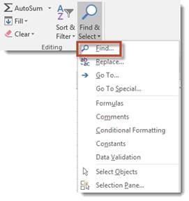
Select Find.
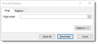
In the "Find What" field, type in the data that you want to find. Maybe it's the word "March."
Select Options to further narrow down the search for the data you need to find.
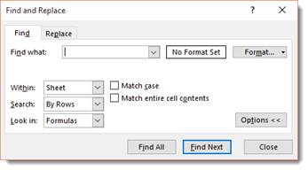
You can now specify where you want to look, such as within a worksheet. You can also search rows or columns � or in formulas.
Click Find All to find all instances of the data. Click Find Next to find the next incident based on the location of the current active cell.
Using Replace
Replace is a lot like Find. The major difference with Replace is you will replace the data you find. For example, maybe you want to replace "March" with "April".
To replace data, go to Find & Select on the Ribbon again. This time, choose Replace.
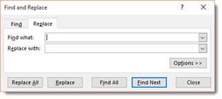
Click Options for more options.
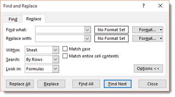
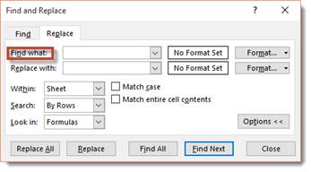
Select the data you want to find in The "Find What" field.
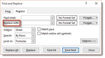
In the "Replace With" field, enter what the data you want to enter as the replacement.
You can choose to replace throughout a worksheet or workbook, you can search by columns and rows, and you can look in formulas, etc.
Next, you can decide how you want to replace. You can click the Find Next button to find the next occurrence, then click Replace after you decide you want to replace it.
You can click Find All to find all occurrences of the data you want to replace.
You can also Replace All to replace all occurrences.
The Go To Feature
Using the Go To feature, you can ask MS Excel 2016 to go to a certain cell. This saves time over scrolling through a worksheet.
To use Go To, go to the Home tab, then select Find & Select again. Now, choose Go To.
When you select Go To, this dialogue box will appear:
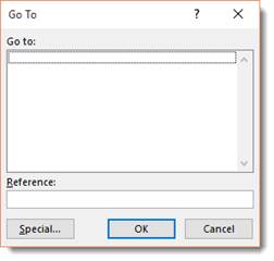
Type in the name of the Column (For example, A), then the number of the row (For example, 3). When you type A3 in the box, then click OK, Excel will take us to A3 automatically. The cell will be selected.
Smart Lookup
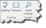
The Smart Lookup button replaces the Research button under the Review tab.
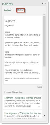
When you click the Smart Lookup button, the Insights task pane will open on the right side of your worksheet.

In this pane, you will find information about the content of the active cell.
If you want a definition for the content of the current cell, click the Define tab in the Insights task pane.
Undo and Redo
Let's say you accidently delete something or deleted it and then decided that you want it back. You grit your teeth and start to grumble, trying to remember the exact data you've entered. It's a lost cause, right? Wrong. The makers of Excel anticipated this problem and supplied an easy solution. The Undo button!
The Undo button is on the Quick Access Toolbar. It looks like this: 
You can click the downward arrow beside the Undo button to determine how many steps backward you want to take with your undo.
The Redo button is to the right of the Undo button. It looks like this: 
The redo button allows you redo an action that you just undid or to repeat the last action by clicking the downward button just as you did with the Undo button.
If Excel cannot redo the last action, the button will be faded.
Locking Rows and Columns by Splitting Panes
When you split panes, you can scroll in the two areas of the worksheet that you've locked, but the non-scrolled areas remain visible. You do this by locking columns or rows � or even both.
For example, you can lock a column so that column remains visible as you scroll to the right in a worksheet. This may be helpful if you have dozens of columns of data, but you still want to be able to view the row labels. By freezing the column that contains the row labels, you can scroll to the right in the worksheet as far as you want, and you will still be able to see the row labels.
-
To lock rows, select the row below where you want the split to appear.
-
To lock columns, select the column to the right of where you want the split to appear.
-
To lock both rows and columns, select the cell below and to the right of where you want the split to appear.
In this example, we're going to split a column.
First, select the column that you want to split. We want to lock column B so we can scroll as far to the right as want in our data and still see our labels. To lock column B, we select the column to the right of it � or column C.
Now, go to the View tab and click Split in the Window group.
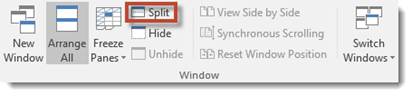
The split is then added to your worksheet. You can see the grey bar in the snapshot below. The grey bar lets you know the columns are split.
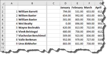
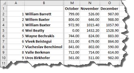
Now we can scroll over to the right, but we can still see our labels:
Locking Rows and Columns by Freezing Panes
When you freeze panes, you select rows and columns that remain visible when you scroll in the worksheet. You freeze panes to keep row and column labels visible as you scroll through.
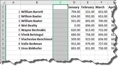
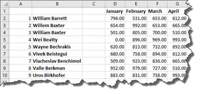
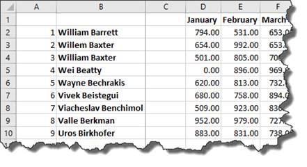
The screenshot below shows a worksheet before we lock and freeze panes.
Let's say we want to freeze the first column. We want to freeze the first column so that we can still see it as we scroll to the right.
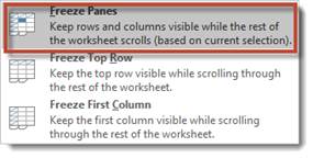
To do this, go to the View tab and click Freeze Panes in the Window group.
You will see this dropdown menu:
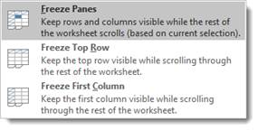
Using our example, we want to freeze the second column. We've already selected the column that comes after the column we want to freeze, which is Column C. We want to freeze column B. Once the column is selected, you can click on Freeze Panes in the dropdown menu.
When we do this, a line appears after Column B.
To unfreeze, follow the same steps, but select Unfreeze Panes.
NOTE: If you choose Freeze First Column from the dropdown menu, you do not need to select a column first.
Spell Check
As you work on a worksheet or after you complete it, naturally you'll want to check it for typos and misspelled words. Excel 2016 will help you check your worksheets for typos and misspelled words using a feature called Spell Check. Now, keep in mind, Spell Check should never be used as a substitute for proofreading it yourself because there are some mistakes that it won't catch, but it is an excellent helper and shortens editing time.
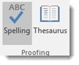
To use Spell Check, click on the Review tab then Spelling in the Proofing group.
If any errors appear in your worksheet, you'll see this dialogue box:
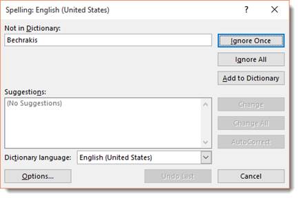
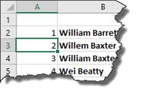
As you can see in the dialogue box above, Spell Check caught a word it didn't recognize, because it's not in Excel's dictionary. You can see the word in the "Not in Dictionary" field.
Once Excel finds a word it doesn't recognize, it will suggest an alternate spelling � if there is one. The alternate spelling will appear in the "Suggestions" field. If the word you entered is simply misspelled, you will likely see the correct spelling in the "Suggestions" field. Simply click on the correct spelling, then click on the Change button to correct it. If you want to correct all instances of the word, click Change All.
Let's go back to the "Not in Dictionary" field for a second. Let's say the word in the field is spelled correctly. Using our example, the word is actually someone's last name, and we've spelled it correctly. The only reason Excel caught it as a possible error is because the word isn't in its dictionary. To keep the word � and leave it spelled as is, click the Ignore button. You can also click the Ignore Now button to ignore all instances of the word. This way, Spell Check won't bring it up as a possible error again.
If you want to add a word to the dictionary, click the Options button at the bottom left of the dialogue box.
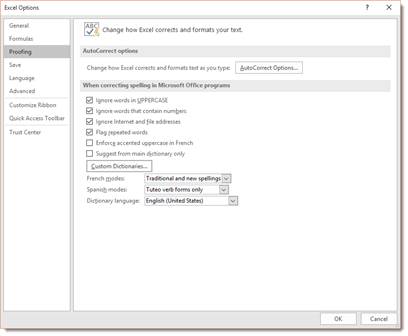
Click Proofing on the left if the dialogue box doesn't open to Proofing by default.
This window allows you to pick a dictionary language and to also add a word to the Excel 2016 dictionary. To add a word to the dictionary, click the Custom Dictionaries button.

You will then see the Custom Dictionaries dialogue box.
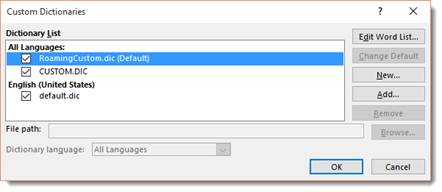
Click the Edit Word List button.
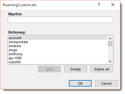
Type the new word in the Words field, then click the Add button.
Click OK.
Keep clicking OK until you get back to the Spell Check dialogue box.
AutoCorrect
AutoCorrect is a feature that allows Excel to automatically correct some errors you make as you type.
To see how it works, let's go back to the Excel Options dialogue box. You can get there by clicking File and going to the Backstage area, then clicking Options on the left.
Click the Proofing tab again.
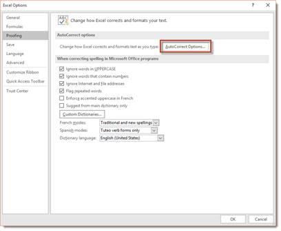
Click on the AutoCorrect Options button (as pictured above) and you'll see AutoCorrect dialogue box.
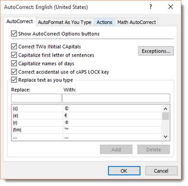
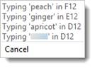
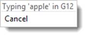
This dialogue box will allow you to program Spell Check and Excel to automatically correct some errors for you as you type. You can also use it to add symbols. In the dialogue box above, you can see that we can add the copyright symbol by simply typing ( c ).
Simply type the word that you want corrected in the Replace field, then type how you want Excel to correct it in the With field. For example, maybe you want to replace "cemetary" with "cemetery".
Track Changes
Have you ever edited something, then realized you liked it better the way it was? Or have you ever edited something someone else wrote and wished there were a way to communicate your thoughts without typing in their document or worksheet? If either of these situations has ever applied to you, then learning how to use Track Changes and Comments in Excel 2016 will appeal to you.
Track Changes gives you the ability to edit or change data in the worksheet and make note of those changes. Excel 2016 will make note of the changes by highlighting the outside of the cell with a different color.
In the upper left hand corner of the cell, an inverted triangle will also appear. Clicking on that will tell you exactly what changes have been made so you know what you've added, what you've deleted, and what formatting changes you have made. This also helps when you have several people changing and editing a workbook.
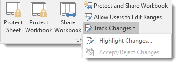
To turn on Track Changes in Excel 2016, go to the Review tab and click Track changes in the Changes group, then select Highlight Changes.
You will then see the Highlight Changes dialogue box.
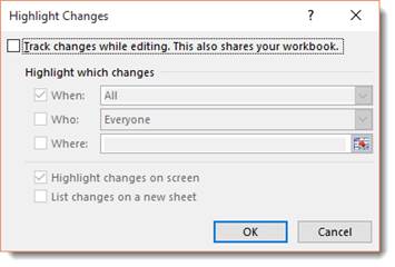
Put a check mark in the box beside "Track Changes While Editing�"
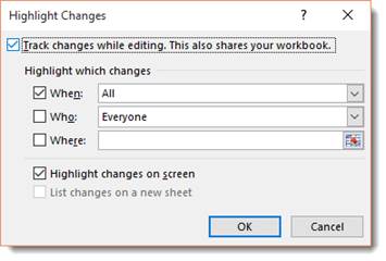
Then, you can select when, who, and where at in the worksheet that you want to track changes.
-
When tells Excel which changes to highlight. We've chosen all changes.
-
Who tells Excel whose changes to highlight. We've chosen everyone who can edit the document. Each user who makes changes to a workbook will be assigned a color by Excel 2016. For example, Mary's changes may show as a cell highlighted in red, Joe's in blue, etc. These are assigned by default. You cannot assign colors to users. When you click on the triangle in the upper left hand corner of a cell where changes have been made, the user's initials will appear. This is another way to let you know who made what changes.
-
Where tells Excel where in the spreadsheet you want to highlight changes. When you put a checkmark beside Where, you can enter in cells or a range of cells.
The highlight changes on screen box should be checked, unless you want the changes listed on a new sheet.
Click OK.
Accept or Reject Changes
Whenever you or someone else makes a change to a worksheet using Track Changes, you can then decide whether to accept or reject the change.
To do this, go to the Review tab, click Track Changes, then select Accept/Reject Changes.
This dialogue box will appear:
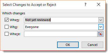
You can select when the changes were made that you want to accept or reject, whose changes you want to look at in order to accept or reject, and where at in the worksheet that you want to review changes.
Click OK when you've selected which changes.
A new dialogue box will appear:
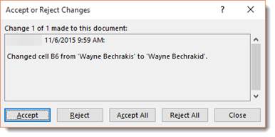
It shows who made the change, what change was made, then gives you the option to accept the change, reject it, accept all changes made in the worksheet, or reject all of them.
Comments
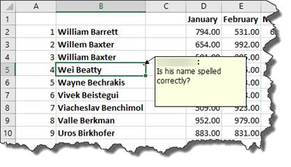
You can also add comments in individual cells in a worksheet to question the data or provide some other input. Excel 2016 will make note that a comment was inserted into the worksheet by placing a red triangle in the upper right hand corner of the cell where it was added. The comment will appear in a pop up box near that cell, as in the example below:
To add a comment, select the cell where you want to add a comment.
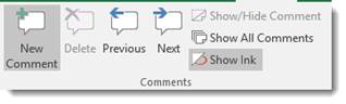
Go to the Review tab and click New Comment in the Comments group.
The box will appear where you can type your comment. Hit Enter to save the comment.

A cell that has a comment in it will have a little inverted triangle in the upper right hand corner:

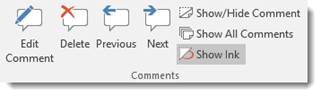
By going back to the Comments group under the Review tab, you can edit comments, delete comments, scroll back to previous comments, or forward to additional comments. You can also choose to show or hide all comments.