The IF function helps to determine what will be displayed to those who view your worksheets in Excel. Because of its purpose, it's one of the most important functions you will learn. IF functions can be used to add comments to your data. They can also be used to hide errors in calculations.
In this article, we will learn about:
-
The IF function
-
The IFNA and IFERROR functions
-
Nesting IF functions
-
The AND operator
-
The OR operator
-
The NOT operator
-
Displaying formulas from one cell in another
About the IF Function
The syntax for the IF function is =IF. This lets Excel know that it is an IF function.
Then, we begin the formula that Excel will use to produce the results we want.
We start with an opening bracket:

Next, we add the evaluation criteria. For example, is six greater than three? The evaluation criteria asks a question. The question has two outcomes. If the answer (or outcome) is correct, such as "Yes, six is greater than three," then the answer is true. If not it is false.
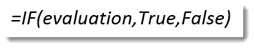
If it's true, we put what happens when the answer is true.
If it's false, we put what happens when it's false.
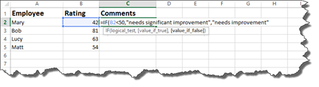
In the worksheet below, we have a list of employees, followed by the rating they received as part of their annual review.
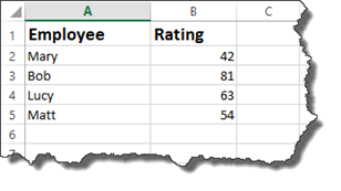
Now, we want to add another column called Comments. In this column, we want to add comments about the scores. This way, when a manager looks at the worksheet, he/she doesn't need to worry themselves with the actual rating � and what that means. They can simply look in comments.
To add a comment based on the rating, we are going to use the IF function.
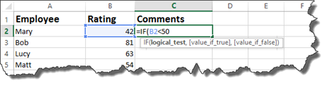
We have started the formula in the snapshot above.
We have said if the employee's rating is less than fifty�
Now we enter what happens.
If it is correct that the employee's rating is less than fifty, the comment should be "needs significant improvement. However, if it's false and if the rating is not less than fifty, the comment should be needs improvement.
Notice that we use quotation marks to enter the comments into the formula.
Now, add an end bracket, then push Enter.
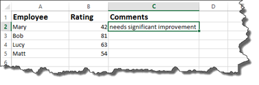
Since this contains a formula where all are cell references are relative, you can use the handle in the lower right corner of the cell, then drag it down to complete the comments for the other employees.
You can also use the IF function to hide Excel error messages.
Let's show you what we mean by taking a look at the worksheet below.
In this worksheet, we have a formula that will divide cell C2 by cell D2.
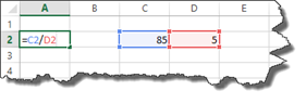
If we push enter in cell A2, it will give us the answer.
However, let's say the data in cell D2 is missing.
When we push Enter, we see an error message.
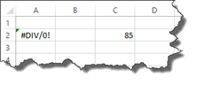
We can use the IF function to hide this error message.
To do this, we write the formula below:
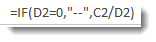
Let's translate what it says. If D2 equals 0, enter two dashes into cell A2 where we have our formula. If it doesn't equal zero, then go ahead and divide cell C2 by D2.
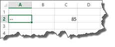
If we would put the number five back into cell D2 and leave the IF formula in place, we would see the answer to C2/D2.
Here's our worksheet below. We have hidden the error message with two dashes.
NOTE: All of the IF functions appear under the Formulas tab and by clicking the Logical button. From there, you can access the Function Arguments dialogue box.
The IFNA and IFERROR Functions
The IFNA function tells Excel what to do if an #NA error is produced, whereas the isna tells Excel what to do if the returned value is #NA.
The #NA error appears in a cell when a value is not available to a formula.
If in our worksheet below, we wanted to find the mode, we would enter this formula:

When we push Enter, the result is displayed.

However, if we went back and changed the second instance of the number four to a six, we would see an #NA error because the value needed is not available to determine the mode.

To avoid #NA values from appearing, we could use the new IFNA function.
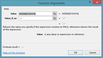
It would be entered like this:

All of the IF functions appear under the Formulas tab and by clicking the Logical button. The easiest way to use the IFNA function is to click the Logical button, then select IFNA.
Below you can see the dialogue box for the IFNA function.
The IFERROR function can be used as a general "cover all" for any errors that might appear in your data. You can use it to specify what will be entered if any error occurs in the calculation of a formula.
It is written the same way as an IF function. However, instead of writing IF, you would write IFERROR. You can access the dialogue box for IFERROR by going to the Logical button under the Formulas tab.
Nesting IF Statements
Just as with VLOOKUPs and HLOOKUPs, you can nest an IF statement within an IF statement.
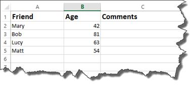
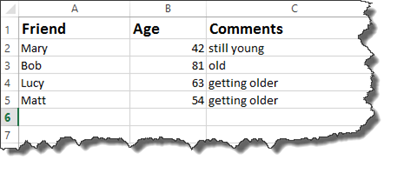
In our worksheet below, we have a list of friends, along with their ages.
We could create a simple IF formula to enter comments.
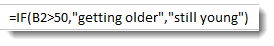
This says if the age is greater than 50, then the comment is getting older. If it's less than 50, then they're still young.
If we nest an IF statement within the current IF statement, we would keep the evaluation criteria, but we would replace one of the outcomes with our new IF statement. However, keep in mind, then when you nest an IF statement, you do not need another equal sign.
Take a look at our new formula below:
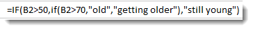
We have our original IF statement intact. We have highlighted the first part of it below.
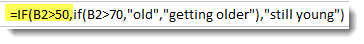
If the age is greater than 50, followed by the two outcomes.
As you can see in our formula above, the TRUE outcome has another IF statement.
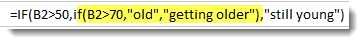
The nested IF statement tells Excel that if the age is greater than 70, enter the comment "old." If it's not, enter getting older.
Our worksheet is shown below with the nested IF statements determining what comment is displayed.
Now, let's break this down into easy to understand terms.
When you enter the formula above with a nested IF statement, Excel reads the first IF statement. It looks at your criteria, then the outcomes for the criteria.
If the outcome for the first IF statement is true, Excel is then going to perform another IF statement to determine what appears in the comments. It will put "old" if the age is greater than 70. It will put getting older if it's not greater than 70. It's very important to remember that these two outcomes both serve as your TRUE outcome for the first IF function.
Now, if your original IF statement returns a FALSE outcome, then Excel will enter "still young."
A nested IF statement gives you a way to enter more than one response for an outcome.
We used a nested if statement for the TRUE outcome. However, you can also use a nested IF statement for a FALSE outcome.
If the nested IF statements are still confusing to you, remember it this way: the nested IF statement provides two additional outcomes for either the TRUE or FALSE outcome of your original IF statement.
Using the AND Operator in an IF Statement
You use the AND operator within an IF statement if you have more than one criteria that needs to be true. Using the AND operator can sometimes be easier to write than multiple nested IF statements.
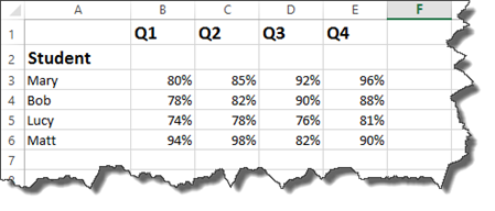
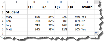
Take a look at the worksheet below.
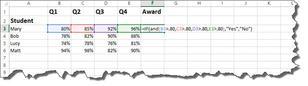
In it, we have a list of students and their grades for the four grading periods.

Each student must have earned greater than 80% in each quarter in order to receive an award. We will use the AND operator to set this as criteria.
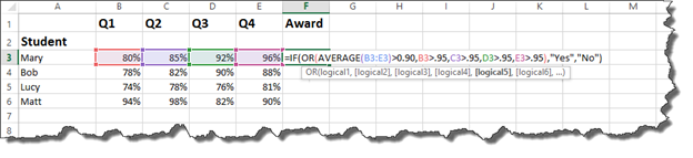
Take a look at how at the formula bar to see how we wrote this.
Now, let's examine it.
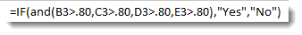
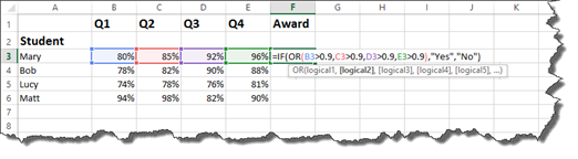
We start out by starting the IF statement with =IF, then the open bracket.
Next, we write AND for the AND operator. The criteria then is placed within brackets. Notice that we have four sets of criteria. The criteria is that each quarter's grades must be greater than 80%. Also notice that all percentages have been converted to decimals when entered in as criteria.
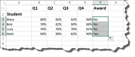
After you've entered the criteria in brackets, you can enter your TRUE and FALSE values. We want the cell to display "Yes" if the criteria is met. We want it do display "No" if it is not met. We then type in an end bracket to close the IF statement.
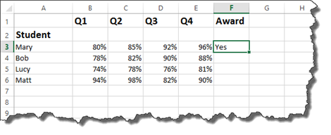
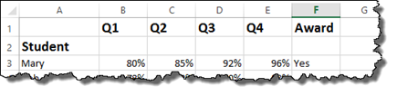
Press Enter.
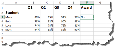
As you can see above, student Mary had one grade that was 80%. All of the grades had to be above 80% to meet our criteria, so a NO was returned.
You can now drag the handle in the cell down to complete the worksheet for all students.
Using the OR Operator in an IF Statement
The OR operator works in the same way as the AND, except it says if one of the criteria listed is true, then the outcome for TRUE is what is displayed.
Let's look at our worksheet.
This time, we want to say if the grade for Q1, Q2, Q3, or Q4 is greater than 90%, then the student gets the award.
You enter it in the same way you did with the IF statement and the AND operator, expect you type OR instead of AND.
Press Enter.
You can then complete the worksheet.
Now let's make it a bit more complicated.
Now we want to say that in order to get the award, the average of all four quarters must be greater than 90% OR at least one of the quarters must be greater than 95%.
In other words, the average of the quarters must be greater than 90%. Or Q1, Q2, Q3, or Q4 must be higher than 95%.
This is the perfect time for you to test your ability writing formulas by entering the formula into the cell.
Press Enter.
Using the NOT Operator
The NOT operator is used in conjunction with the AND or OR operator.
The best way to explain how the NOT operator works is to show you the NOT operator in action.
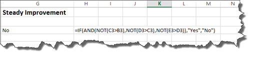
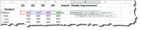
Working with our students and grades again, we want to determine if the grades have improved each quarter.
To do that, we are going to use the IF statement with the AND operator since we are using multiple criteria.
We will use the NOT operator to make sure Q1 is not higher than Q2. Q2 must be greater than Q1.
In addition, Q3 must be greater than Q2, and Q4 must be greater than Q3.
We've started the write it below:
Let's finish.
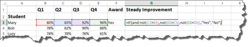
Hit Enter.
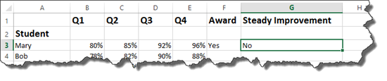
We can see there is not steady improvement.
Remember: The NOT Operator is used within AND or IF options. You must use the NOT operator for each piece of criteria. You cannot type in the NOT operator once, then use it for all criteria.
Displaying Cell Formulas In Another Cell
Starting with Excel 2013, you can display the formula from one cell in another. In our worksheets so far, we could view the formula in a cell by double clicking on the cell. However, once we pressed Enter or tabbed out of a cell, we couldn't see the formula unless we looked in the Formula Bar.
To display a formula from one cell in another cell, go to the cell where you want to formula to appear.
You will use the FORMULATEXT function.
Type the equal sign, followed by formula text.
Enter an open bracket, then click the cell that contains the formula you want to display.
Add the closing bracket.
For our example, we are going to display the formula in cell G3 in sell H3.
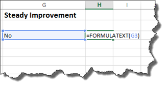
Press Enter.