A pivot table is a tool that you can use to summarize data when you have a lot of it in a worksheet. A pivot table can count totals, give an average of the data, or sort data – in addition to other things. In this article, we are going to go in-depth as we learn to create and work with pivot tables.

We will discuss how to:

• Use Recommended PivotTables

• Create a pivot table from scratch

• Format a pivot table

• Create multiple pivot tables

• Move a pivot table

• Delete a pivot table

• Use filters

• Sort data in a pivot table

• Refresh data in a pivot table

• Verify data in a pivot table

Recommended Pivot Tables is a feature that is new to Excel 2013. With Recommended Pivot Tables, Excel analyzes the data that you have in your spreadsheet, then suggests possible pivot tables for you to use.

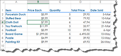
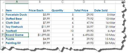
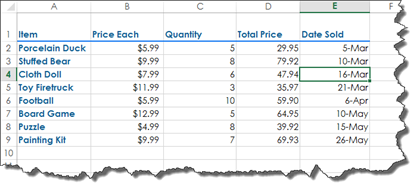
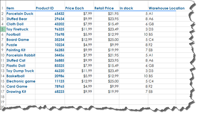
Take a look at our worksheet below:

This worksheet is simply a list of items, the price for each item, the quantity sold, the total price, and then the date sold.

To see the recommended pivot tables, click anywhere in the worksheet.                                                                                                                   

Go to the Insert tab, then click Recommended Pivot Tables in the Tables group.

You will then see the Recommended PivotTables dialogue box.

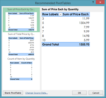
In the dialogue box, you will see Excel's recommended PivotTables.

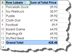
As you can see, in our recommended pivot tables, Excel summarizes the data by the price of each item, the total price, and the number of items.

If you want to use one of these suggested pivot tables, simply click on the pivot tables in the column on the left. 

We have chosen the total price for each item.

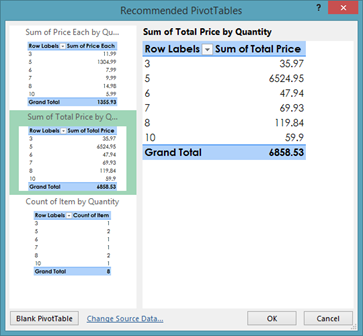
That pivot table is now visible in the right column.

Click the OK button.

The pivot table is then placed into a new sheet, as shown below.

Creating a PivotTable from Scratch

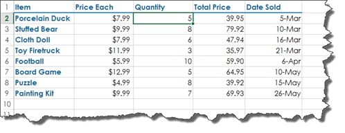
We are going to use the same worksheet that we used when working with Recommended PivotTables. It is pictured below.

In starting to create your own pivot table, you do not need to select or highlight data. The only way that you would be required to select data is if you had a blank column or row within your data. Of course, you wouldn't want that included in your pivot table, so you would select the data you did want included.

To start creating your pivot table, click within the data, then go to the Insert tab. Click the PivotTable button.

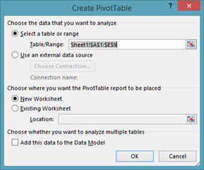
In the Select a Table or Range field, Excel fills in the range of cells that contains your data.

You can compare the range of cells listed above with our worksheet, and you can see that all the data was included. Unless you need to change the range of cells, you do not need to enter anything into this field.

Next, decide if you want the new pivot table to appear in the existing worksheet (with your data) or in a new worksheet.   It's recommended that you place it into a different worksheet, but the choice is ultimately yours.   If you place it in the existing worksheet, you'll need to specify the location where you want to place it.

Click OK.

This is what you will see in a new worksheet:

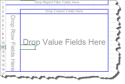
This is where your pivot table will start.

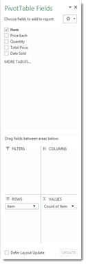
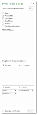
If you look to the far right side of the Excel window, you will see PivotTable Fields, as shown below.

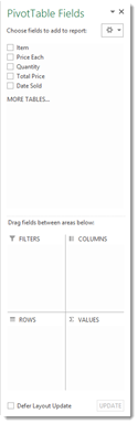
You will use this to create your pivot table. 

In the top section, you will see your columns listed.

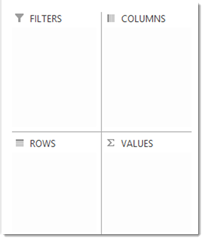
The bottom section contains the sections of your pivot table.

• Filters is the filter above the pivot table.

• Columns are the column headings.

• Rows are row headings.

• Values are the crossover of the rows and columns.

The only thing in the bottom section that you need to make a pivot table work is Values. You'll find that Rows, Columns, and Filters help to organize the data and information in the pivot table.

To see what we mean, let's choose a column from the top half.

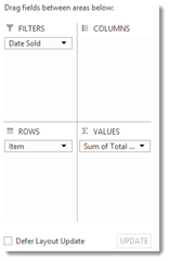
We are going to choose Item. We want each item to appear in a row, so we drag it to the Rows section in the bottom half. 

Next, we are going to click on Items in the top half again, and drag it to the Values section.

All you have to do is drag and drop.

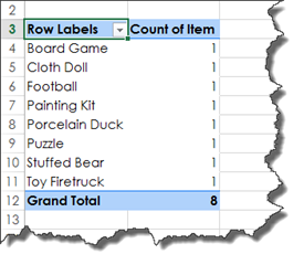
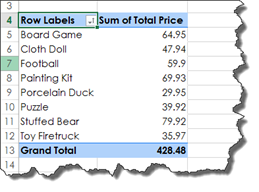
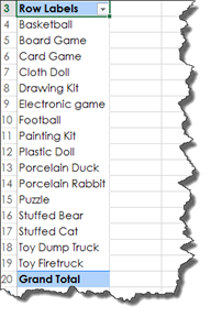
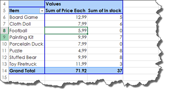
Now, if we look at our pivot table, we see that Excel has summarized the number of each item in our worksheet.   Remember, this is the number of times the item appears in our data. It's not an inventory count.

Now let's say we want to add another column to our pivot table.  

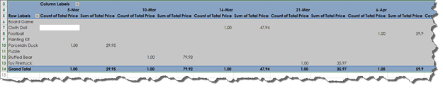
We are going to drag Date Sold from the top section to the Columns section in the bottom half, as shown in the snapshot below.

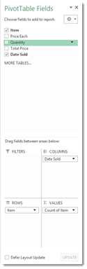
Take a look at our pivot table:

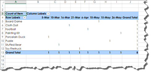
Now we can see which item sold in which months. 

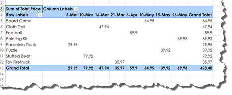
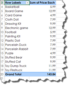
With pivot tables, there's something you need to keep in mind. If you drop a text field (such as Item) into values, Excel will assume you want to count the values. We did this, and it counted the number of occurrences of the item in our data.   If you drop a numerical field into Values, Excel will assume you want a sum of the items.

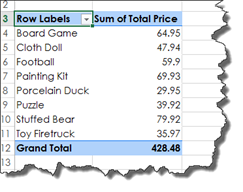
We've redone our pivot table by dragging Total Price into the Values section (and removing Item).

If you make a mistake and drag something into Values, Columns, Filters, or Rows that you don't want there, you can simply click and drag it back to the top section. This will remove it. 

You can also drag and drop to and from Values, Columns, Rows, and Filters. 

You can do these things to create the pivot table that you want.

Changing the Formatting and Formulas of PivotTables

It's easy to create a pivot table in Excel 2013, but that's just where the fun begins.   Now that you created a pivot table, it's time to learn how to format it.

Below is our pivot table.

If you wanted to format the data in the pivot table, you could do so by selecting a column or row, then going to the Home tab and applying formatting, such as changing the font type, font size, or font color. Those are very basic Excel skills and easy enough for you to do.

However, if you applied formatting in this manner, if you ever refreshed the data in your pivot table or added rows or columns, the formatting might not be applied.

Instead, go to the panel on the right side of the Excel window where we created the pivot table. In the bottom section of the pivot table, click the downward arrow to the right of the field you want to format.

In the snapshot below, we are going to click the downward arrow to the right of the Item field.

Click on Field Settings, as circled in red above to format the field.

However, in order to show you a better example, we are going to click on the field Sum of Total Price in the Values section, then choose Field Settings from the menu.

We then see the Value Field Settings dialogue box. 

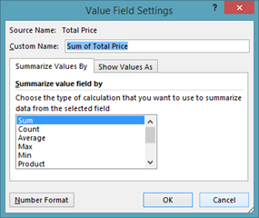
In this dialogue box, we can change the name of the field in the pivot table by going to the Custom Name field.

Right now, we have the cells in this field formatted so that all numbers display as currency. If we wanted to change that, we would click the Number Format button.

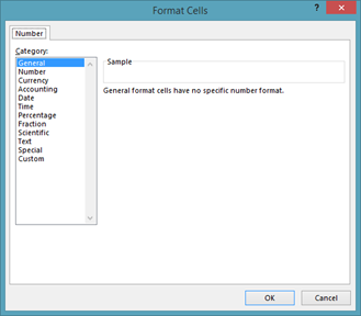
Choose the formatting for our cells, then click OK.

This will return you to the Value Field Settings dialogue box. 

Also in the Value Field Settings dialogue box, we can change the function.   Right now, we have it at the default, which is Sum.   It can be changed to Count, Average, Max, Min, etc. All of these functions relate to the total price.   For example, average of the total price, and so on.

Click OK when you are finished.

You can also add the same field more than once.  

This means that, if you wanted, you could change the function for the Total Price field to Count.   Then, you could drag the Total Price field to the Values section again, which would display the Sum of Total Price.

Just make sure you change the number format that matches the function.   We wouldn't want Currency for the Count function, for example.

As you can see in our pivot table pictured below, you now have columns for the Count and Sum functions. 

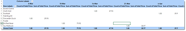
Creating Different PivotTables Using the Same Data

You can create as many pivot tables as you need to using the same data from the same worksheet.  You can choose to place the pivot tables together, or you can place them in different worksheets.

We are going to create another pivot table by clicking in the data, then going to Insert>PivotTable.

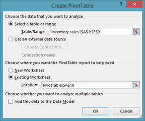
As you can see in the dialogue box pictured above, we have chosen to place the new pivot table in the same worksheet as the pivot table that we created earlier in this article.   We did this by choosing Existing Worksheet, then clicking on the tab of the worksheet that contained the pivot table.   Next, we clicked on the cell where we want the upper left hand corner of the pivot table to be placed.

Click OK.

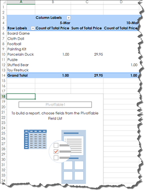
You can now see our new pivot table below our existing pivot table.

Moving PivotTables

You can move a pivot table to a new location within a worksheet or to a new worksheet entirely.

To move a pivot table, click within the data of the pivot table, then click the Analyze tab under PivotTable Tools in the Ribbon, as pictured below.

Next, click Move PivotTable in the Actions group.

NOTE: Some Excel 2013 users may see an Action button instead. In this case, click Action>Move PivotTable.

You will then see this dialogue box:

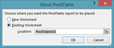
You can choose to move the pivot table to a new worksheet, or you can click on a cell in the existing worksheet where you want to place the pivot table.

Click the OK button when you are finished.

The pivot table is moved for you.

Deleting PivotTables

To delete a pivot table, click within the data, then go to the Analyze tab under PivotTable Tools in the Ribbon.

Click the Select button, then choose Entire PivotTable. 

This selects the PivotTable.

You can then press Delete on your keyboard.

The Report Filter Option

In the snapshot below, we have a simple pivot table.

You can see that we have dragged and dropped the Item field into the Rows section, and the Total Price field into the Values section in order to create the pivot table.

Now we are going to learn what happens when you drag a field to the Filters section.

For this example, we are going to drag the Date Sold field to the Filters section.

When we do this, we can see the filter is added above our pivot table.

If we click the downward arrow to the right of Date Sold, we see our filtering options:

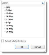
We can now filter the data in our pivot table by the date the items were sold.

Of course, we can also add another filter to our pivot table to further refine the data that's summarized in the table.

Let's drag the Quantity Field to the Filters section.

If we go to the pivot table and click the dropdown arrow beside Quantity, we can choose a quantity to filter the data by.

Click OK when you've chosen how you want to filter the data.

You will then see the changes to your pivot table.

Sorting Data in a PivotTable

Data in a pivot table can be sorted by row or column labels, as well as values.

Whenever you create a pivot table, Excel does the sorting for you.   Excel puts row and column labels in the order that they appeared in the original data worksheet. 

If you want to sort row or column labels, simply click the dropdown arrow that appears to the right of either Row Labels or Column labels.

You can see Row Labels circled in red below.

We are going to click the downward arrow. 

As you can see in the next snapshot, we are now given the ability to sort the labels alphabetically from A to Z, or Z to A.

We are going to click on Sort A to Z.

Now, if you want to sort values in a pivot table, click the downward arrow again. 

This time, click on More Sort Options.

You will then see the following dialogue box.

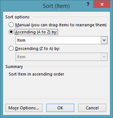
Choose if you want to sort the values from A to Z or Z to A by putting a check beside your choice.

Next, click the downward arrow in the field below your choice, as shown below.

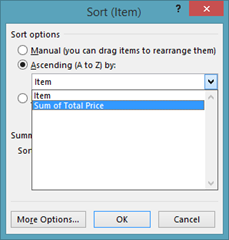
In the snapshot above, you see that we can also sort by Sum of Total Price – or our values.

Select the option, then click OK.

Our data is then sorted by values.

Refreshing the Data in a PivotTable

A pivot table is based on data that is contained in a worksheet.   If you change the data in the worksheet after you have created a pivot table, you will need to refresh the data in the pivot table so that it reflects the current data in the original worksheet.

Let's show you what we mean so that it makes sense.

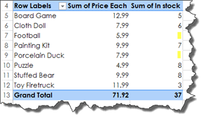
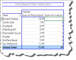
Below is our pivot table.

Now, we are going to go back to our original worksheet.  

Let's say, as an example, that there has been a price increase for the porcelain duck.   It is currently $5.99, but we are now going to make in $7.99.   To change that data, all we have to do is click in the cell, then make the change.

However, when we go back to our pivot table, our Sum of Price Each column still reflects the $5.99 per unit pricing.

We need to refresh the data so the changes made in the original data are reflected in our pivot table.

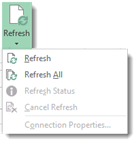
To do this, go to the Analyze tab under PivotTable Tools.   Go to Refresh>Refresh All. 

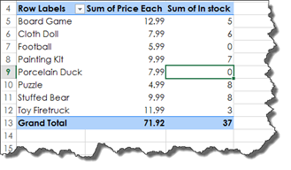
As you can see, the data in our pivot table is now refreshed.

Another thing you can do to make sure that your data stays refreshed is to set your options in Excel so that the data in your pivot table is refreshed each time you open the workbook. 

To do this, go to the Analyze tab again.

Click the Options button in the PivotTable group.

You will then see this dialogue box:

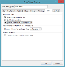
Click the Data tab.

Put a checkmark beside Refresh Data When Opening the File, then click OK.

Verifying the Data in a PivotTable

It's easy to take for granted that the data presented in a pivot table is correct.  

However, if you ever wanted to double check to make sure that the data is correct, there is an easy way to do that.

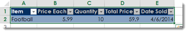
Let's say we want to verify that the price of the football is really $5.99.

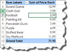
To do this, double click on the cell that contains the value that you want to double check. In this case, it's the cell we've selected above.

When you double click on the cell, Excel pulls up all the data that it used to come up with this number. 

In our case, it's the row entry for the football. However, if the value you clicked on used multiple bits of data, it would list all the data that it used to produce the value.

 

Continuing to Work with PivotTables

PivotTables are an invaluable tool in Excel because they give you a way to summarize data; however, they also give you a way to look at the exact data that you need. Let's face it. Worksheets can contain tons of data.   You may have a worksheet that contains a list of employees, the departments they work in, their job titles, the location where they work, and their salary – and there may be 1500 employees.   By using a pivot table, you can easily view only the employees who work in the Accounting Department in your Denver, Colorado location (as an example). 

That said, there is so much to learn about PivotTables that we are going to continue to talk about them in this section. We are going to discover how to:

• Add multiple fields to columns and rows

• Work with grand totals and subtotals

• Adjust empty cells

• Create groups

• Use the classic way to create pivot tables

• Apply PivotTable styles

• Create custom styles

• Create calculated fields

• Use the timeline filter option

• Filter data using the data slicer

• Import data from a SQL server

Adding Multiple Fields to Columns and Rows to a PivotTable

In all the pivot table examples thus far, we have used only one field per column or row. However, we can also add multiple fields to columns and rows.

Below is our data.

Now we are going to create a pivot table by going to the Insert tab, then clicking the PivotTable button.

We are going to place our pivot table in a new worksheet.

To start with, we are going to add the Item field as a row in our pivot table.

We are going to add the Price Each field to the Values section.

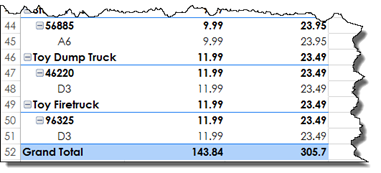
Now, we want to add another field to our rows. We want to add the Product ID. To do that, we are going to drag the Product ID field to Row section and place it beneath Item, as shown below.

We also want to add the warehouse location of each item, so we are going to drag that to the Row section as well.

Take a look at our pivot table:

We now have Item as the heading for each row, then Product ID and Warehouse Location for subheadings.

Now, let's add another value. Let's add Retail Price.

You can add as many additional fields as you want to your rows and columns. 

Grand Totals and Subtotals in PivotTables

Grand totals are always displayed by default in Excel 2013. If you look at the bottom of our pivot table, you will see the grand total:

If you do not want grand totals displayed, you can turn them off by going to the Analyze tab under PivotTable tools, then Options.

Click the Totals & Filters tab.

You can then uncheck Show Grand Total for Rows and/or Show Grand Totals for Columns.

Subtotals are also automatically displayed in our pivot table. 

If you don't want subtotals to appear, right click on the field label. In our example above, it's Basketball. 

Select Field Settings.

As you can see, Subtotals are turned on by default (Automatic).

Put a check beside None, then click OK.

Of course, you can always choose to present the subtotals using a different function.   You can choose Count, Average, Product, and etc. by putting a check beside Custom, then clicking OK.

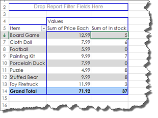
About Empty Cells in PivotTables

Sometimes you may see empty cells appear in your pivot table. We have highlighted such cells in our pivot table below.

You may wish to make it so that a 0 appears in those cells rather than having them appear blank.

To do this, click anywhere in the pivot table, then right click.

Select PivotTable options, then go to the Layout & Format tab.

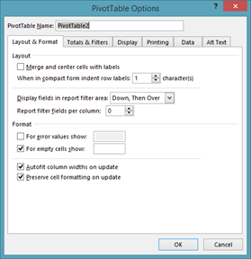
Go to the Format section.

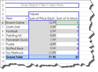
Put a checkmark beside For Empty Cells Show, then enter a 0 in the box.

Click OK.

As you can see, zeros now appear in the empty cells.

Manual Grouping

You can also group things together in your pivot table.

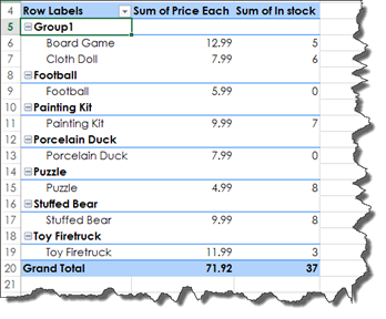
Let's say in our pivot table that we want to group together the board game and the cloth doll. 

We are going to select those.

Now, we are going to go to the Analyze tab, then click Group Selection.

You can now see Group1 in our pivot table.  

If we compress the group, it will show us a subtotal.

Take a look at our pivot table again. Notice that when we put the two items into a group, the rest of the items are listed as groups as well, even if none of them are grouped together.

To rename a group, select the group, then rename it in the Formula Bar.

Another Way to Create PivotTables

Here's another way to create PivotTables without having to drag different fields into different sections of the PivotTable Fields panel.

Go to the Analyze tab, then click Options.

Click the Display tab.

Put a checkmark beside Classic PivotTable Layout, then click OK.

Now you can drag fields from the PivotTable Fields panel right onto your pivot table.

Working with PivotTable Styles

The PivotTable styles are found under the Design tab of the PivotTable tools. You can see this tab when you click anywhere in your pivot table. 

A style will apply formatting to your pivot table.   It can change the color, font, and other attributes.

The different pivot table styles are pictured below in the Ribbon.

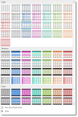
You can simply mouseover any of these styles to see how it will look when applied to your pivot table.

This is the style that we have chosen:

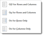
Based on the style that you choose, you may be able to turn row headers on or off by adding or removing the checkmark in the Ribbon.

The same is true for column headers. We have chosen to turn ours off since they were on by default so that you can see the difference.

You can also choose if you want banded rows:

Or banded columns:

In addition to applying a style, we can also choose the report layout.

To do this, click the Report Layout button under the Design tab.

You can click on the different layouts to see how they affect your pivot table.

By clicking the Subtotals button under the Design tab, we can chose if and how subtotals are displayed.

By clicking the Grand Totals button under the Design tab, we can choose our preference for how grand totals are displayed.

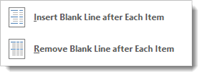
By clicking on the Blank Row button under the Design tab, we can insert blank rows to make our pivot table easier to read.

Creating a Custom PivotTable Style

If you do not want to use a built-in PivotTable style, you can create your own style using the tools provided in Excel 2013.

To do this, go to PivotTable Styles in the Design tab. Select New PivotTable Style from the dropdown menu.

You will then see the New PivotTable Style dialogue box.

Start out by entering a name for the style.

Now what you need to do is format each aspect of the pivot table.

We are going to start with the first column. Click on First Column, as we've done below.

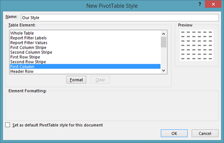
Now click the Format button.

Under the font tab, set your font type, style, and size.   You can also choose your font color.

Click the Border tab.

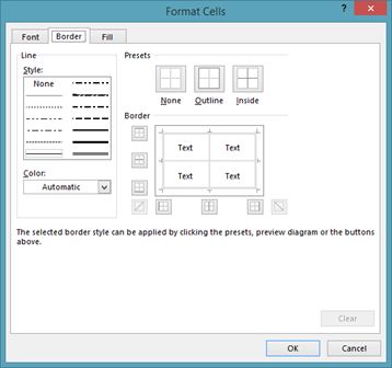
Choose the border style that you want, as well as where the border appears.

Next, click the Fill tab.

Choose a fill color for the column.

When you are finished, click the OK button.

This takes us back to the New PivotTable Style dialogue box.

First Column now appears in bold print to let us know that we have chosen formatting for it.

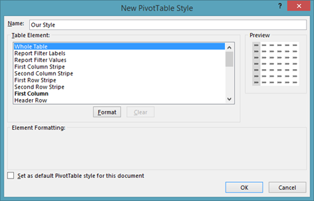
Now let's click on Whole Table, then click the Format button.

Follow the same steps again.   Repeat the steps until you have your new style created, then click OK in the New PivotTable Style dialogue box.

Your new style will then appear in the PivotTable Styles under the Design tab.

Click on it to apply it to your pivot table.

Creating Calculated Fields

Calculations can be done within a pivot table without having to access the original data. 

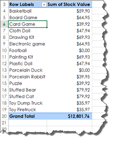
In our pivot table below, we have our items listed.   We haven't added any values to the table yet, because we want to calculate the value of all the items in stock in our pivot table.

To do this, we are going to add a calculated field. Click on Fields, Items, & Sets under the Analyze tab, then select Calculated Field.

We then see the Insert Calculated Field dialogue box.

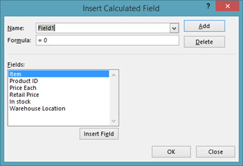
Enter a name for the field.

Next, create a formula for the field. Do so by clicking the fields from the Fields list.

We are going to select Price Each, followed by the operator for multiply, then In Stock.

Now click OK.

The Timeline Filter Option

The timeline is new in Excel 2013. Whenever you have dates included in your original data, you can use the timeline to help further sort your data – without adding those dates to your pivot table.

Let's show you what we mean.

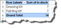
Take a look at our pivot table below.

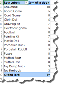
We have our items and the quantity we have in stock.

We want to find out the dates on which we received each item.   We don't have this information as a row or column in our pivot table, but it's in our original data from which we created the pivot table.

To view the timeline and be able to filter by the dates, we are going to click in our pivot table, then go to the Analyze tab.

Click Insert Timeline.

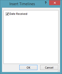
As you can see, we only have one field in our original data that contains dates, so we put a checkmark beside it, then click OK.

We can now see our timeline.

It is shown as a floating window in our worksheet.

Next, click on a month in the timeline – or select multiple months – to filter the data.

The Data Slicer

The data slicer provides another way to filter data in your pivot table. The slicer allows you to choose any fields in your data, then use that as a filter in the pivot table. You can use any of the fields in your original data to filter the data in your pivot table.

To add a slicer to a pivot table, click inside your pivot table, then click Insert Slider under the Analyze tab.

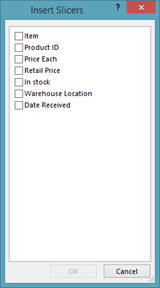
Put a checkmark beside the fields you want to use to filter the pivot table and for which you want the slicers created, then click OK.

We chose Retail Price.

Once the slicers are created, filter the data by selecting the items you want to display in each slicer by clicking them. 

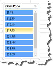
We now see our filtered results in the pivot table.

Using Data from a SQL Server

So far, we have used pivot tables that used data from the same workbook. We can also create a pivot table from an external database, such as an SQL server.

To do this, we are going to create a blank worksheet, then go to the Data tab.

Click the From Other Sources button, and select From SQL Server.

You will then see the Data Connection Wizard.

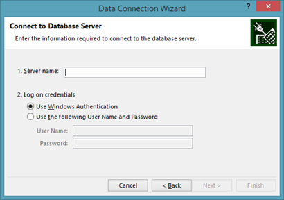
Enter your information to connect to your SQL server.

Click Next.

In the next window, you will see a list of the data available on the server.

Select that data you want to use, then click Next.

This brings you to the final window. In this window, Excel will give your data a file name. This is because Excel will save the connection if you want to use it again in the future.

Click Finish.

You will then see the Import Data dialogue box.

In the Select How You Want to Use this Data In Your Workbook section, choose PivotTable Report.

Choose if you want to place it in an existing worksheet or a new worksheet.

Now you will see your fields in the PivotTable Fields panel on the right side of your Excel window. 

You can now follow the same steps you learned earlier in this article to create a pivot table. However, instead of using the data from the workbook, it will use the data you have imported from your SQL server.