With all the functions and formulas Excel 2013 allows you to use in worksheets and workbooks, there's little doubt that you are going to have some errors.   If you have a lot of data contained in your worksheets and workbooks, it can be a chore to go back and isolate each error, then take steps to fix it. Finding and fixing errors could wind up being just as time consuming as entering and calculating the data. At least, it would be if Excel 2013 didn't offer you the tools you need to help you efficiently audit and troubleshoot your workbooks and data.

In this article, we will take a look at how you can:

• Add and remove tracer arrows to trace data and formulas.

• Use Error Checking to find errors

• Find and correct circular references

• Use Trace Error

• Use step-by-step formula processing

• Use the Watch Window

About Tracer Arrows

Tracer arrows allow you to trace problems in a worksheet. If there are errors in formulas or things aren't working as they should within your worksheet, tracer arrows can help you find the problem. They do so by helping you trace "the path" of your data.   Tracer arrows show you how data in one cell is connected to data on other cells. 

In Excel 2013, there are two different types of tracer arrows.

• Dependent tracer arrows show you which cells are dependent upon the value in the cell you've selected.  They show you the cells that come AFTER the cell you've selected and our dependent on the data from the cell you've selected. 

• Precedent tracer arrows work in the opposite way. They show you what cells feed into the cell you've selected. The cell where the arrow starts is the first cell that feeds into the cell you selected.   The arrow ends in the cell you selected.

Adding or Removing Tracer Arrows

Adding and removing tracer arrows is easier than it may sound.   We are going to first cover how to add dependent tracer arrows, followed by precedent tracer arrows, as well as how to remove them.

Take a look at our worksheet below.

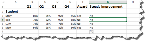
We want to find out which cells are dependent on G4.

To do this, we are going to go to the Formulas tab. 

Go to the Auditing section, and click Trace Dependents.

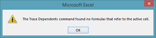
As you can see, we get a message that there aren't any formulas that refer to the active cell.

Instead, let's click on cell B3, then click Trace Dependents.

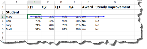
We can now see all the cells that are dependent on cell B3. 

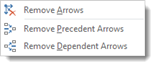
To remove a dependent tracer arrow, go to Remove Arrows in the Auditing group under the Formulas tab and click the downward arrow beside it. From the dropdown menu, choose Remove Dependent Arrows. If you select Remove Arrows, it will remove both Dependent and Precedent arrows.

To add a precedent tracer arrow, click a cell. Remember, Excel will show you all cells that feed into the one you've clicked.

We are going to select G4 again.

Go to the Formulas tab. Click Trace Precedents in the Auditing group.

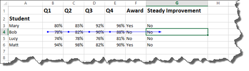
You can now see which cells feed into cell G4.

To remove a precedent tracer arrow, go to Remove Arrows in the Auditing group under the Formulas tab and click the downward arrow beside it. From the dropdown menu, choose Remove Precedent Arrows. 

Using Error Checking

Excel gives you quite a few ways to audit your worksheets and check for errors.   The first way is using Error Checking. Error Checking points out all of the errors that may occur in cells or formulas in cells, then allows you to get help with the error, ignore the error, copy the formula from the cell, or edit the formula in the Formula Bar.

To use Error Checking, go to the Formulas tab, then click the downward arrow beside Error Checking in the Formula Auditing group.

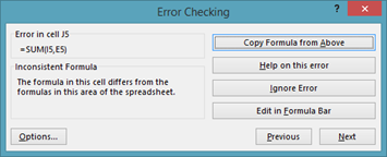
As you can see, Excel pulls up the first cell where there is an error.   It tells us the error exists because of an inconsistent formula.   If we look in our worksheet and pull up the cell above it which uses the same formula, we can see there is indeed an error. The sum should be calculated for E5,I5. Instead, it's showing as I5,E5.

Let's go back to Error Checking.

If we click on Copy Formula from Above, it will copy the formula from the cell above it.

This fixed our error. 

For the time being, however, we are going to reproduce the error to show you what your other options are with Error Checking.

This time, let's click on Help On This Error.

The Excel 2013 Help files will open.

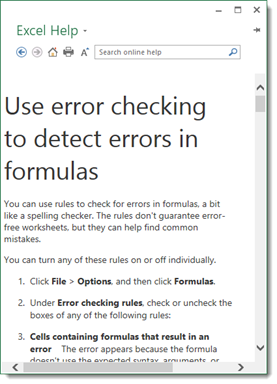
This is very generalized help about using Error Checking in Excel.

The next button is Ignore Error.   If you click this button, the error will be left in the worksheet.

The final button is Edit in Formula Bar. This enables you to correct the formula in the Formula Bar.

If you click Next, it will take you to the next arrow in the worksheet.

We are going to click the Copy Formula from Above button again to fix the error.

Finding and Correcting Circular Reference Errors

In Excel 2013, a circular reference is an error that occurs when a cell is dependent on itself to calculate a formula, so it is unable to display the result of the calculation in the cell.

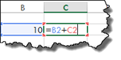
Here is an example. We want to add B2 plus C2.   We have placed the formula inside C2, which means C2 is where we want the result displayed.

When we push Enter, look at what happens.

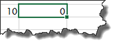
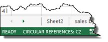
A zero appears in the cell. At the bottom of the spreadsheet, we see that a circular reference has occurred.

 We can also go to Circular References in the Error Checking dropdown menu under the Formula tab.

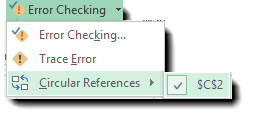
Whenever you error check an Excel worksheet, you can go to Formulas>Error Checking>Circular References to check for circular references.   As you can see above, Excel will show you where there are circular references in your worksheet.   You can click on any that are listed, and Excel will take you to them.

If we click on $C$2, we are taken to our cell.

We can then click the green pop out signal in the upper left hand corner of the cell. It looks like this:

We are offered options to correct the error.

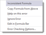
The options we see in this dropdown menu are the same that we encountered in the last section using Error Checking.  

We are going to choose to Copy Formula from Above, and the error is fixed.

Trace Error

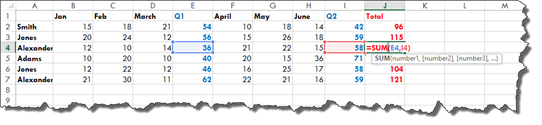
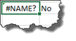
Whenever we see an error in a cell such as #VALUE and #REF, as shown below, we can easily enough fix these types of errors by going to the Error Checking dropdown under the Formulas tab and selecting Trace Error.

This will make either a precedent or dependent trace arrow appear in the worksheet.

In the snapshot above, we have a precedent tracer arrow. We know this because the arrow starts in a cell, then ends in the cell where there's the error.

The precedent tracer arrow lets us know that we may need to check those cells when fixing the error. Once you find and fix the error, the precedent tracer arrow disappears.

Formula Processing

If you have a long formula in Excel, it can be hard to go back and see exactly what the formula is actually doing. 

Take a look at the formula below.

In this formula, you can see that we have a lot going on. We have more than one calculation, plus we have a lot of cell references like C6 and B6.

If we want to see exactly what is going on in the formula as Excel processes the formula step-by-step, we go to the Formulas tab, then click Evaluate Formula in the Formula Auditing Group.

We then see this dialogue box:

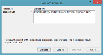
In the dialogue box, we see our formula.   We also see part of the formula is underlined. Click the Evaluate button.

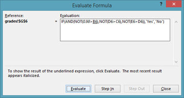
Excel now evaluates the part of the formula that was underlined. We see the data that is in the cell now instead of just the cell reference.

Click the Evaluate button again.

We now see the next thing that is going on in the formula. Again, we see the actual value instead of the cell reference.   In addition, you are seeing in the Evaluate Formula window is the steps Excel takes to process the formula.

Click Evaluate.

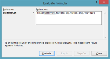
We can go through like this and evaluate each part of the formula to see what is going on.

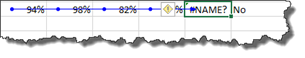
If you click the Step In button, Excel will step in to the part of the formula you are looking at, as shown below.

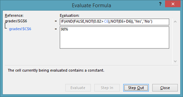
The top field shows us that we have stepped in to C6.

The bottom field shows us that the value in C6 is 98%.

You can then click Step Out and keep evaluating your formula.

As you evaluate your formula by clicking the Evaluate button, you are also watching the steps Excel takes to process your formula.  

As you can see in the snapshot below, Excel as processed and calculated the formula.

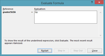
Click the Restart button to evaluate the formula again, or click Close.

The Watch Window in Excel 2013

The Watch Window in Excel 2013 lets you watch particular cells to see if the value in those cells change.

To access the Watch Window, go to the Formulas tab, then click on Watch Window.

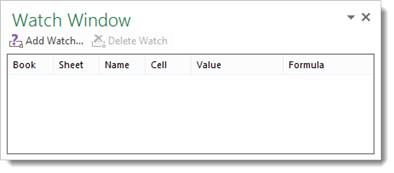
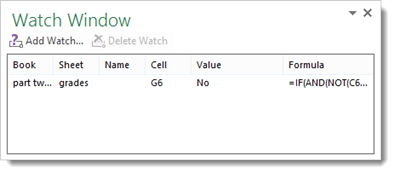
As you can see about, the Watch Window tells you the workbook and worksheet where the cell is located, the name, the actual cell that's being watched, the value of that cell, as well as the formula contained in that cell.   

This allows you not only to watch a cell, but also know exactly where the cell is located, as well as its purpose (for example, to calculate an average).

Because the Watch Window lists workbooks as well as worksheets, you can keep watching cells as you work in other workbooks.   If the data in a watched cell changes, you'll see it in the Watch Window.

You can move the Watch Window around Excel and dock it above, below, or to the side of your worksheet.

This can be helpful as you're checking your workbook for errors.   You can use the Watch Window and see as those errors are being fixed.

The Watch Window is also helpful if you have a formula that uses cells from other worksheets in its calculation.    As you change values of the other cells that feed into the cell you're watching, you can see the value of the watched cell change in the Watch Window.

To add a cell to watch in the Watch Window, select the cell, then click Add Watch in the Watch Window.

You will then see the address of the cell in the Add Watch dialogue box.

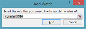
Click Add.

You can then see that cell in the Watch Window.