Excel 2013: How to Use Data Lookups

Data lookup is quite simply the process where values in Excel are scanned until certain results are found. In Excel 2013, there are two main formulas for looking up the data you have in a worksheet. There is VLookup where the V stands for vertical, and there is HLookup where the H stands for Horizontal.

The Basic VLookup Formula

Below is the basic VLookup formula.

Inside the brackets, you will see the information that Excel asks us to enter into the formula.

You can also go to the Formulas tab, click the Lookup & Reference button, then select VLookup.

You will then see this dialogue box:

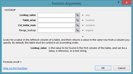
The benefit of using the dialogue box when entering a formula is the bit of instruction that Excel gives you for each field. If you're newer to Excel, it's recommended that you use the Function Arguments dialogue box to create your formulas. It's a lot less trial and error that way.

For the time being, however, let's look the formula in our worksheet again.

Lookup_value is the value that we want to look up.

The table_array is the table where the data will be retrieved. This value can be a range or the name of a range.

Col-index_num is the column number in the table. The first column in your table is column 1.

Range_Lookup is typically true for false. True will give you a near match. If you want to find an exact match, it's false.

Let's learn how to use the VLookup formula.

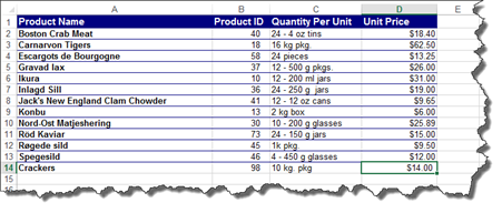
Take a look at our worksheet below.

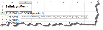
On the left, we have birthdays listed. We know that 12 means December, and we could use the MONTH function to fill in December for us, but instead we want the text value.

On the right, we've created a lookup table. We are going to use a VLookup to find the text value.

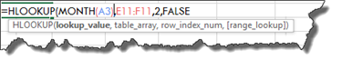
We start by entering the VLOOKUP function, then open brackets.

The first piece of information we must supply is the lookup value. We know the lookup value is the month located in Column A (the first column), but we must use the MONTH function to specify this, as shown below.

Next, we add a comma, then for the table_array, we are going to highlight the cells in the table; however, we don't highlight the column headers.

Enter another comma.

Now, for the col_index_num. Ours is Column 2. We then enter another comma.

Since we want the exact match, we enter FALSE.

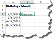
Close the brackets, then push Enter.

About Lookup Tables

A lookup table is created by simply creating a table in Excel. It's used as a master list of sorts, and you will use it to locate data that you need to find using search criteria that you will enter into your lookup formula. You can use a huge table of data that you've created as your lookup table. You do not have to create a lookup table just to use either the VLookup or HLookup functions.

For example, let's say you have a table within a spreadsheet that contains 15,000 customer names, complete with address, billing information, shipping information, anniversary dates, and etc. You can use a lookup formula to find specific data within the table. If you wanted to find the address, for example, you could create a lookup formula to find that within your table of data.

Naming Lookup Table Data

If you're looking up data that may be on different worksheets within a workbook, it makes it easier if you name the data you're going to be searching.

This is easy to do.

Go to the lookup table data. Click anywhere in the data, then press CTRL+A. This selects all of the data.

Next, go to the Formula tab.

Click the Define Name button in the Defined Names group.

Enter a name for the group. The scope is workbook.

Click OK.

Now, when you enter the table_array information into your data lookup, you can simply enter this name. In our case, it's products. You will see it appear in a dropdown menu.

Please note that if you add data to the end of a lookup table after you've named it, then enter the name of the data into Excel (we named ours Products), the formula will not retrieve that data because it is not part of your named data.

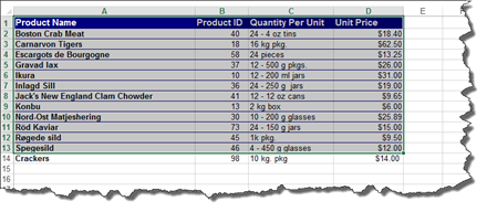
We entered another product to our product list below.

Now we can go to our Name box, and choose the name of your data.

As you can see, the last row is not included.

If you add rows or columns to a lookup table after you've named it, insert the data into the existing data table. Do not put it at the very beginning or the very end. Otherwise, you will have to rename it, then change your lookup formula.

Look what happens when we insert the new row above our last row.

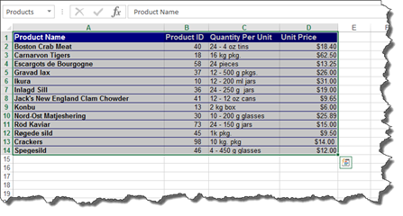
It is now include with the data.

However, you can always add extra blank rows in your lookup table so that you have room to add new things at the end.

VLOOKUP: A Real Example

It's important that you understand exactly how VLOOKUP works. For that reason, we are going to show a more realistic example.

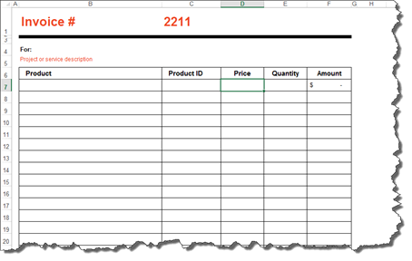
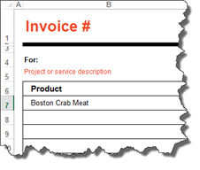
Below we have an Excel invoice. This is just one of the pre-built templates that we are going to use.

We also have a product list in another worksheet.

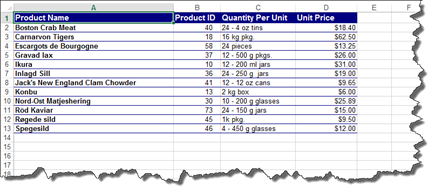
We are going to use VLOOKUP to find the product ID and the price per unit for our invoice.

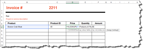
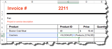
Take a look at our invoice again.

We have entered in Crab Meat as the first product sold.

Now, we are going to use VLOOKUP to find the product ID.

Enter your VLookup formula in the cell for the product ID.

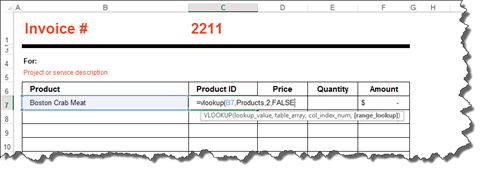
Notice that we entered in Products for the table_array.

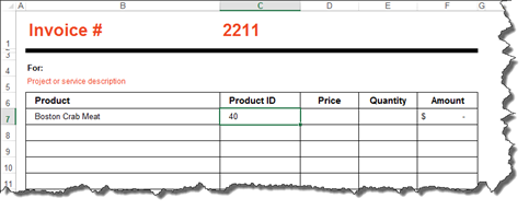
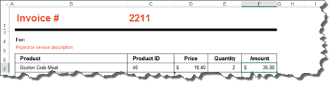
Hit Enter.

You should now have the product ID in the cell.

Now let's do the price.

As we fill in our formula, notice that when we get to table_array and type in the name for our data, it appears in a dropdown list.

Finish entering in the formula.

Close the brackets when you're finished entering the formula, then press Enter.

About HLOOKUP

Whereas VLOOKUP is vertical lookup, HLOOKUP is horizontal lookup. However, vertical or horizontal lookups do not refer to the table in which you want to place the results. Instead, it refers to the table in which you're using to search for data.

When you use the HLOOKUP function, you are looking for data horizontally. In VLOOKUP, we looked in a column for data. Columns are vertical. In HLOOKUP, you search rows. Instead of entering the column number, you will enter the row number, as shown below.

Add the end bracket to the formula, then press Enter.

Working with Near Matches

Let's talk about range lookup in the VLOOKUP and HLOOKUP formulas. As we already have learned, if you enter FALSE as the range lookup, Excel will return the exact match for the results.

However, if you use the TRUE argument for a lookup, it will use the nearest match that is of the next largest value if an exact match is not found.

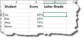
For our lookup table, we have a grading scale.

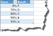
We are going to use VLOOKUP to input the letter grade.

Below is our formula. Notice that we named our data "score."

Hit Enter.

Now, drag the handle in the lower right hand corner of the results cell to fill in the rest of the data.

When There's Missing Data in a Lookup

If you use VLOOKUP or HLOOKUP, and Excel cannot find the data you're looking for, you'll see this message appear in the cell after you press Enter to see results.

What you will want to do if you see this message is to run an IF statement to make sure the data really isn't there.

Let's use our invoice and product list as an example. We are going to create the formula, product the #N/A message, then run the IF statement.

In our invoice below, we've entered a product that we know doesn't exist in our product list.

We are going to hit Enter to see the results of the formula.

As we already knew would happen, Excel can't find the results.

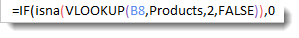
To make sure the lookup is correct, we are going to modify our formula so we can run an IF statement.

To start with, we typed IF after the = for the IF statement, then we entered an opening bracket and typed "isna."

We also added a closing bracket to the end to close the IF statement and our VLOOKUP. As you can see above, our VLOOKUP formula sits inside the "isna" formula.

If the result really is NA, we want Excel to give us 0 as a result because there isn't a product number.

If there is a value, we want it to do a VLOOKUP again, so we copy and paste the VLOOKUP in after placing another comma.

As you can see, we then get a zero because the data is indeed missing.

Nesting a Lookup Within a Lookup

You can nest a lookup within a lookup to go through multiple tables and pull out a value.

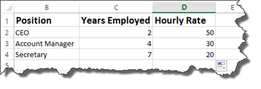
For example, in our worksheet shown below, we have a list of employees with the years that they've worked for our fictional company.

We want to use our lookup tables to determine their hourly rate of pay.

That said, our fictional company determines an employee's hourly pay by their job classification, then the number of years they've been on the job.

We have two data tables for that.

Here is the first. We named it "class."

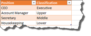
As you can see, this table lists the various job positions in the company, then lists the classification for each position.

Here is our second table. We named it "salary."

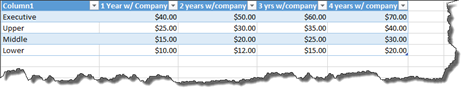
This table lists the different classifications, then the hourly rate of pay for those classifications based on the number of years the employee has been on the job.

To figure out the hourly rate for our worksheet, we will use nested VLOOKUPS.

Let's start out by using VLOOKUP to find the job classification for the first employee in our list.

Now we will nest this VLOOKUP inside another VLOOKUP.

To do this, we will put the cursor after the equal sign in our formula, then type VLOOKUP again, followed by an opening bracket.

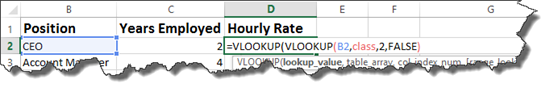
Put a comma after the closing bracket, then enter your table array for the new VLOOKUP, the column number, then FALSE for an exact match – as shown below.