Key Terms
o Synthetic division
Objectives
o Realize that if you know all the zeros of a polynomial, you can find the corresponding algebraic expression for that function
o Be able to factor a polynomial using synthetic division
o Be able to find all the zeros of a polynomial (given sufficient information)
Polynomials of Higher Degree
Factoring can also be applied to polynomials of higher degree, although the process of factoring is often a bit more laborious. Recall that a polynomial of degree n has n zeros, some of which may be the same (degenerate) or which may be complex. Consider the simple polynomial f(x) = x3; this polynomial can be factored as follows.
f(x) = (x)(x)(x)
As we can see from this expression, there are three zeros, all of which are at x = 0. Now, let's reverse our view of factoring a bit to illustrate the principle. Let's say we have a third-degree polynomial p(x) defined below.
p(x) = (x – 1)(x – 2)(x – 3) = (x2 – 3x + 2)(x – 3) = x3 – 6x2 + 11x – 6
Notice that we start with the factored form, which obviously has three zeros (one at x = 1, one at x = 2, and one at x = 3), and then use distributivity of multiplication to find the polynomial expression. Let's take a look at the graph of this function to confirm the location of the zeros.
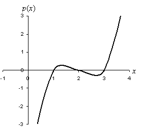

As we can see in the graph, the function crosses the x-axis at x = 1, x = 2, and x = 3. This confirms our assumption that the factored form elucidates the zeros of the function. As a result, we can construct a polynomial of degree n if we know all n zeros. Stated in another way, the n zeros of a polynomial of degree n completely determine that function. This same principle applies to polynomials of degree four and higher.
Practice Problem: Find a polynomial expression for a function that has three zeros: x = 0, x = 3, and x = –1.
Solution: Earlier, we noted that if you know all the zeros, you can find the polynomial. A zero at x = c corresponds to a factor (x – c) in the polynomial. Let's use this fact to construct the polynomial p(x) that corresponds to the zeros given in the problem.
p(x) = (x – 0)(x – 3)(x – (–1)) = x(x – 3)(x + 1)
Now, let's expand this result to find the polynomial expression.
p(x) = x(x2 – 2x – 3) = x3 – 2x2 – 3x
We can confirm the result by either graphing, testing each zero, or both. Let's just test each zero.
p(0) = (0)3 – 2(0)2 – 3(0) = 0
p(3) = (3)3 – 2(3)2 – 3(3) = 27 – 2(9) – 9 = 27 – 18 – 9 = 0
p(–1) = (–1)3 – 2(–1)2 – 3(–1) = –1 – 2 + 3 = 0
This function is equal to zero at each of the corresponding x values.
Factoring Polynomials
Factoring a quadratic function can be a somewhat difficult process, depending on the coefficients of the function. With higher-degree polynomials, factoring can be even more difficult. Note, however, that if we know one of the zeros (say at x = c), we can rewrite a polynomial of degree n as the product of (x – c) and a polynomial of degree n – 1. We can repeat this process (if we know or can find other zeros) until we have completely factored the polynomial. To do this, though, we need an efficient method of finding the lower-degree polynomial when we factor. One method of doing this is synthetic division, which is an algorithm for factoring polynomials. Let's look at this algorithm in the context of the above practice problem. We have p(x) = x3 – 2x2 - 3x, and let's say that we are told that a zero is located at x = 3. Thus, we w–nt to factor p(x) as follows, where p2(x) is a polynomial of degree two.
p(x) = (x – 3)p2(x)
Now, let's consider the algorithm for synthetic division.
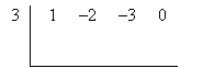

2. Carry the first coefficient. The highest-order coefficient should be carried down below the bracket.

![]()
3. Multiply the value of the zero by the last value you wrote below the bracket and write it under the next coefficient inside the bracket. You will then add the values in this column and write the value under the bracket in the same column.
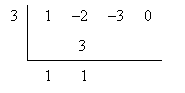

4. Repeat step 3 until you reach the end of the bracket. The final number that you write under the bracket should be zero-if not, either you have made a mistake, or the zero value outside the bracket is not truly a zero of the polynomial.
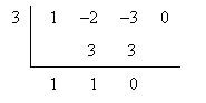

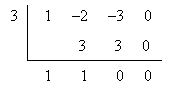

5. Write the new factored polynomial. Use the zero value outside the bracket to write the (x – c) factor, and use the numbers under the bracket as the coefficients for the new polynomial, which has a degree of one less than the polynomial you started with.
p(x) = (x – 3)(x2 + x)
Because the example used in the presentation of the synthetic division algorithm above now includes only a quadratic polynomial, we can factor without performing another synthetic division.
p(x) = (x – 3)(x)(x + 1)
The zeros of this polynomial are 3, 0, and –1, as we expected. Thus, synthetic division can allow us to factor polynomials of an arbitrary degree.
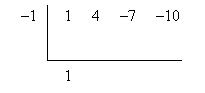
Practice Problem: Find the zeros of the polynomial p(x) = x4 + 4x3 – 7x2 – 10x if one of the zeros is at x = –1.
Solution: Before we do anything difficult, notice one simple fact about the polynomial p(x): each term has at least a factor of x. So, let's factor x out to start.
p(x) = x4 + 4x3 – 7x2 – 10x = (x)(x3 + 4x2 – 7x – 10)
So, we know that x = 0 is a zero of the function. The problem also tells us that there is a zero at x = –1; let's use this to factor (x + 1) out of the remaining third-degree polynomial using synthetic division. First, we set up the division using the value of the zero and the coefficients of the polynomial. We'll also carry the first term.

We'll now run through the algorithm to find the factored polynomial.
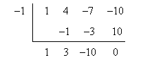

The (partially) factored polynomial is then the following.
p(x) = (x)(x3 + 4x2 – 7x – 10) = (x)(x + 1)(x2 + 3x – 10)
We now have a quadratic that we can factor using less sophisticated methods.
p(x) = (x)(x + 1)(x2 + 3x – 10) = (x)(x + 1)(x + 5)(x – 2)
We now can see all of the zeros of the polynomial: x = –5, x = –1, x = 0, and x = 2. Let's plot a graph of the function to check our results.
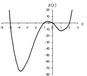

Note the x-intercepts (zeros) of the function, which correspond to what we found by factoring.
Practice Problem: A particle has a velocity with respect to time that obeys a third-degree polynomial function. If the particle is at rest at 0, 2, and 3 seconds, find the polynomial function that describes the velocity of that particle.
Solution: This is a word problem that forces us to synthesize various aspects of what we've learned already with some of the other skills we should already have. First, note that the problem wants us to find a function that describes the velocity of a particle as a function of time. Let's call this function v(t), where t is time in seconds. The function v(t) is a third-degree polynomial.
The problem statement also informs us that the particle is at rest (that is, it has zero velocity) at t = 0, 2, and 3 seconds. These t values correspond to the zeros of the function; using this information, we can construct v(t).
v(t) = (t)(t – 2)(t – 3)
Now we can expand the result.
v(t) = t(t2 – 5t + 6) = t3 – 5t2 + 6t
We can test the result by substituting the t values that correspond to the zeros of the function.
v(0) = (0)3 – 5(0)2 + 6(0) = 0
v(2) = (2)3 – 5(2)2 + 6(2) = 8 – 5(4) + 12 = 8 – 20 + 12 = 0
v(3) = (3)3 – 5(3)2 + 6(3) = 27 – 5(9) + 18 = 27 – 45 + 18 = 0
The result checks out.