Entering and managing lots of data can be a daunting task.  It's easy to get overwhelmed in all of those rows and columns of information.  The solution is to use a form.  A form is simply a dialog box that lets you display or enter information one record (or row) at a time.  It can also make the information more visually appealing and easier to understand.

Most people who are familiar with the MS Office suite associate complex forms with Excel's sister program Access, but you can use them in Excel as well.  In fact, you can even share data between the two programs.

There are two kinds of forms available in MS Excel: data forms and worksheet forms. 

·       Data forms are generally used for data entry.  They are simple forms that list the contents of a single column.  What's more, they can display up to 32 fields at a time.  This is especially helpful when dealing with a data range that reaches across more columns than will fit on a screen.  You can insert, alter, delete, and even find records with data forms.

·       Worksheet forms are more sophisticated and specialized.  They can be customized to fit the information at hand or to fill a particular need.  They can even be complex and appealing enough to be printed or distributed online.  Worksheet forms must be created using the Microsoft Visual Basic Editor.

Using a Data Form

Before you can use the data form function in MS Excel, you must first create a label at the top of each column for each range of information.  That's because Excel uses these labels to create fields on the form.  See the illustration below for an example of a simple data form.

 

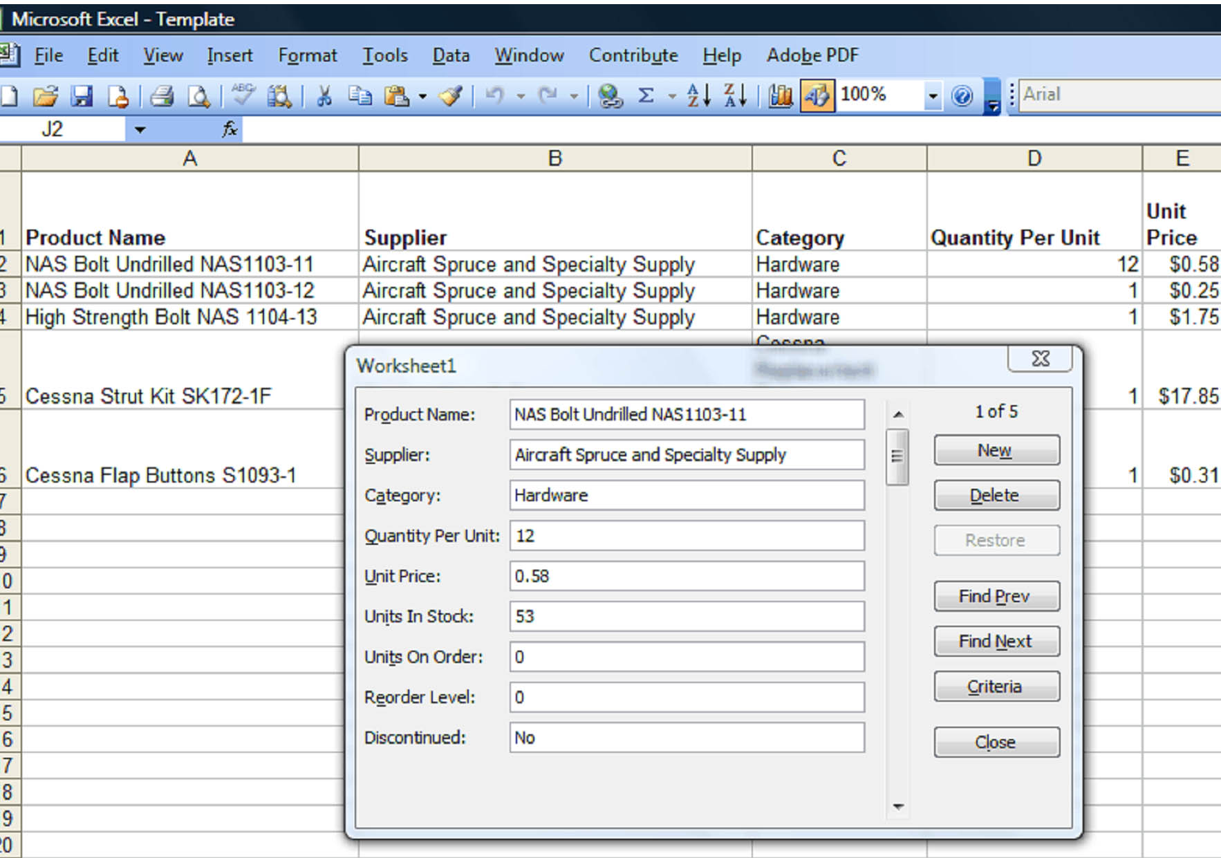
To access the data form function, select a cell in a data range and click Data > Form.  You will see a window much like the one above.  The title at the top of the window tells you where you are.  In this case, on Worksheet1. 

Entering Data Using a Data Form

If you've ever filled out an application online, you're familiar with a data form.  In fact, when you fill out one of those applications, you are inserting information into a database program much like Excel. 

Entering data is as easy as selecting the correct field and typing.  Use the Tab key to jump to the next field.  When you are finished, press Enter.  This automatically takes you to the next record.  If you are at the end of the record list, it will create a new file. 

Use the arrow keys or the Find Prev, Find Next buttons to browse through records.

Data Validation

Data Validation let's you choose what information is acceptable to enter into a cell.  For instance, you may have a product code that has four digits.  You can set up a cell so that anything other than a 4-digit number will display an error message.

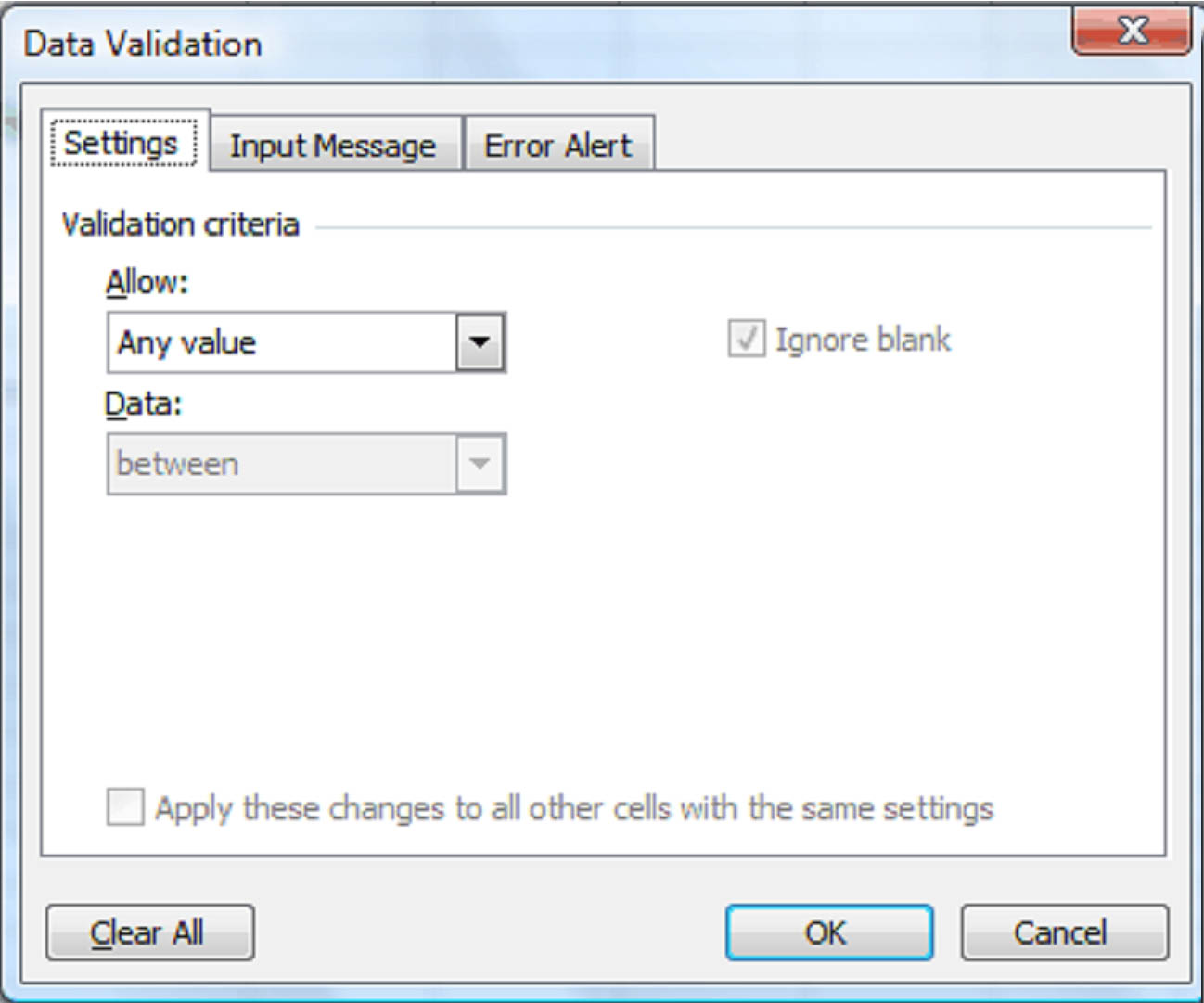
To set up data validation, select a cell and click Data > Validation.  You will see a window that looks like this.

 

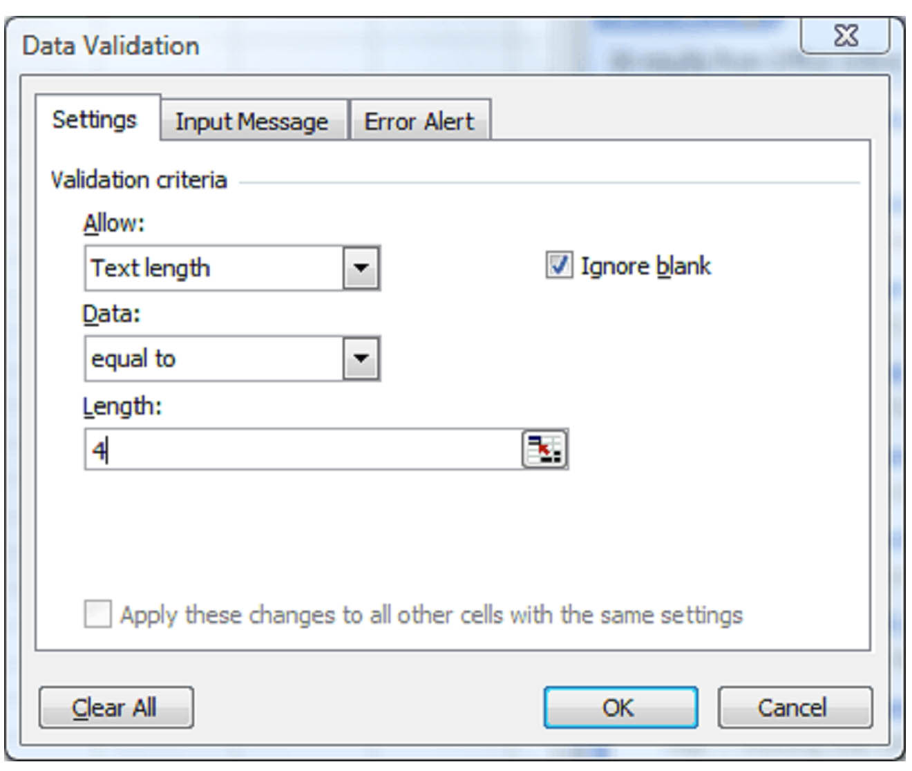
Since we're going to set up a cell to accept only a 4-digit number, we will select Text length from the drop down menu that says "Allow" over it.  From the Data dropdown menu, we are going to select "equal to" and in the length text field we will type "4."  That tells Excel we want an entry with four characters.

 

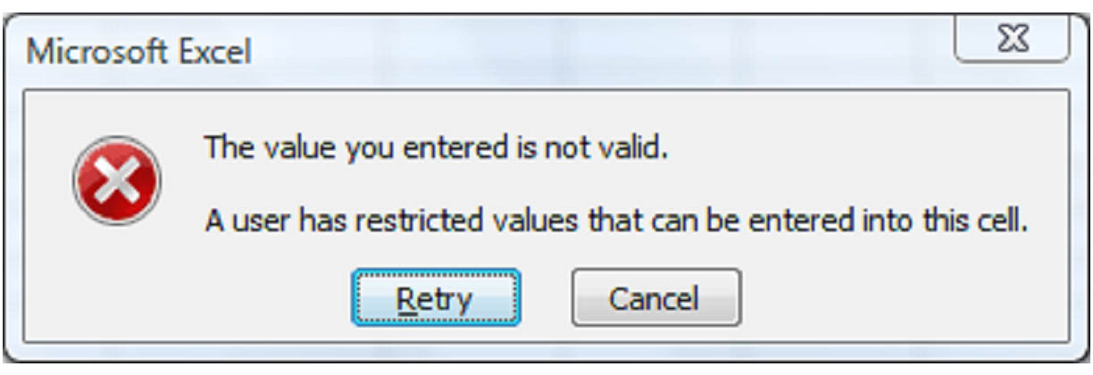
From here, we can hit OK and have Excel provide a generic warning that looks like this:

 

Alternatively, we can create a custom warning by selecting the Error Alert tab.  Which looks like this:

 

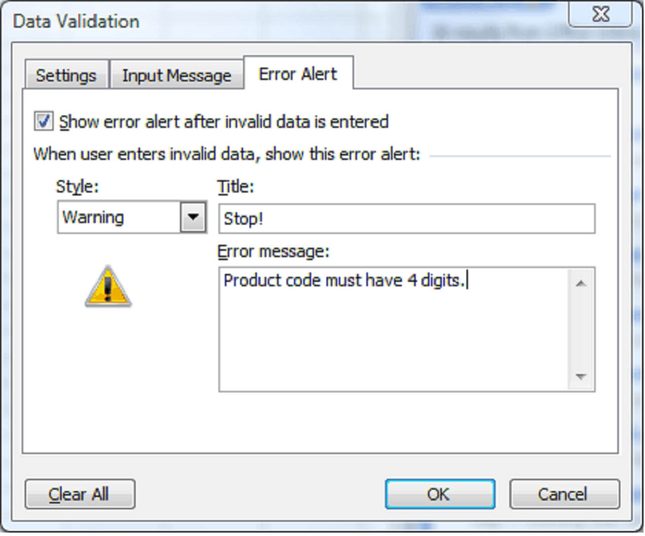
Here we have selected the Warning style and entered the text for our error alert.  When a user enters a code of less or greater than four digits, the message will look like this:

 

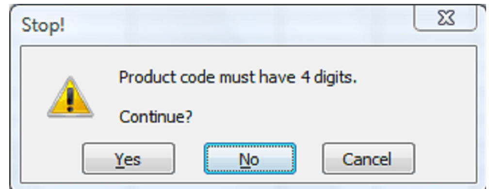
There are three kinds of error messages available in Excel: information messages, warning messages, and stop messages.  Information messages and warning messages do not prevent invalid information to be entered into the cell; they simply inform the user that such an entry has been made.  Users can choose to ignore the warning.  A stop message, on the other hand, will not all an invalid entry.  It has two buttons, Cancel and Retry.  Cancel restores the cell to its original value, and retry returns them to the cell for further editing.

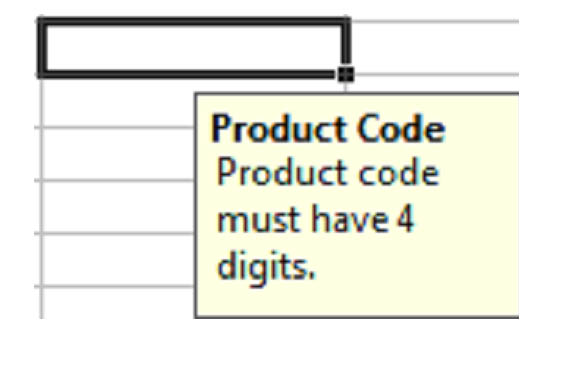
You can also set up a message to remind users what the restrictions or expectations are.  Use the Input Message tab to create a custom reminder.  It will display anytime the cell or the range of cells is selected, as in the example below.

 

Auditing

MS Excel 2003 gives you a variety of tools to audit information in a worksheet.  Just like data forms, formula auditing can take some of the confusion and frustration out of dealing with lots of different formulas.  You can also see which cells have invalid information in them.  To use these tools, you must first launch the formula auditing toolbar.

 

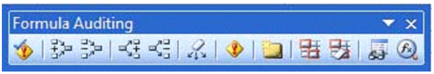
Since we've just been talking about validation, let's take a look at the two buttons that will allow you too see if invalid entries were made in any cells.  These buttons are:.  The button on the left will put a red circle around any invalid entry in the workbook.  The button on the right will remove the circle.

 

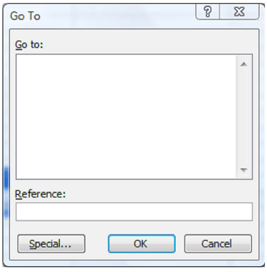
It is not always apparent which cells have formulas in them.  Therefore, the first step to evaluate the formulas is to find them.  To do this, select Edit > Go To and then click Special in the bottom left hand corner of the Go To window.

 

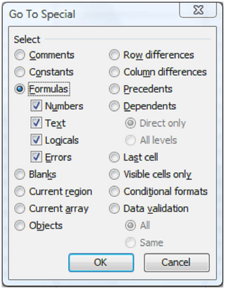
Then select the Formulas button in the Go To Special Window.

 

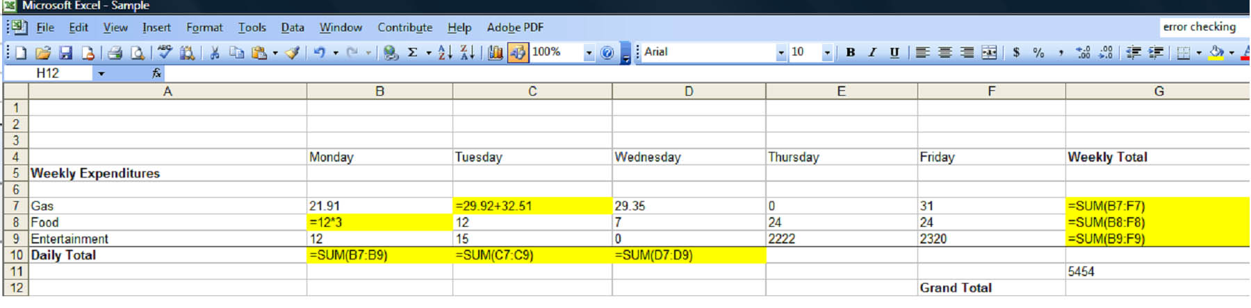
As you can see in the example below, the whole numbers will be changed to the formulas and the formula cells will be selected.  To make it easier to see the cells when they are no longer selected, you can click the fill button .  This will fill the selected cells with very visible yellow.  When you are finished auditing formulas, you can select the cells again by using the Go To Special process and remove the fill.  All of the highlighted cells below contain formulas.

 

Let's take a closer look at the other functions on the Formula Auditing toolbar.  The first is the Check Errors function .  This button does exactly what its name implies:  it checks the formulas for errors.  If it finds one, it will alert you.

The next two buttons  allow you to trace (and turn off trace) precedents in a formula.  A precedent cell is one that is referred to by a formula in another cell.  For instance, in the following example we've selected G9 and turned on Trace Precedents. 

 

B9 thru F9 are precedents because they are referred to in the formula in cell G9.  As you can see, the trace precedents button shows you the relationship between the cells.

The next group of buttons  turn on and off the trace dependents function.  A dependent cell is one that contains formulas that refer to other cells.  In the following example we've selected cell C8 and turned on the trace dependents function.  The blue arrows point to the cells that depend upon the value in cell C8.

 

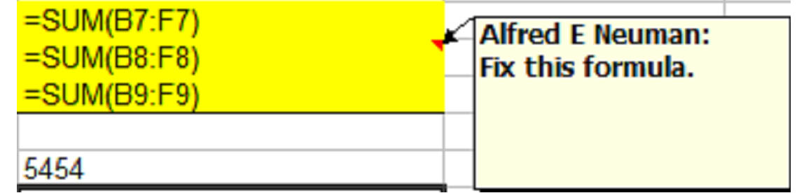
The next button removes all arrows in the document.    You can attach a comment to any cell by clicking the comment button .  When a comment is made, a red wedge appears in the corner of the cell it's attached to.  Place your mouse pointer over the cell to see the comment.

 

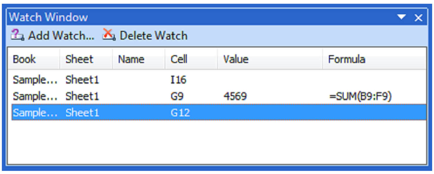
The watch window is useful when you're not sure if alterations to the value in a cell will affect a formula.  You can easily remind yourself of the formula by adding it to the watch window.

 

The Evaluate Formula function will perform the calculations of a formula in slow motion so you can see each step.  To use it, select a formula, then click the evaluate formula button  in the toolbar.  You will see a box that looks like this:

 

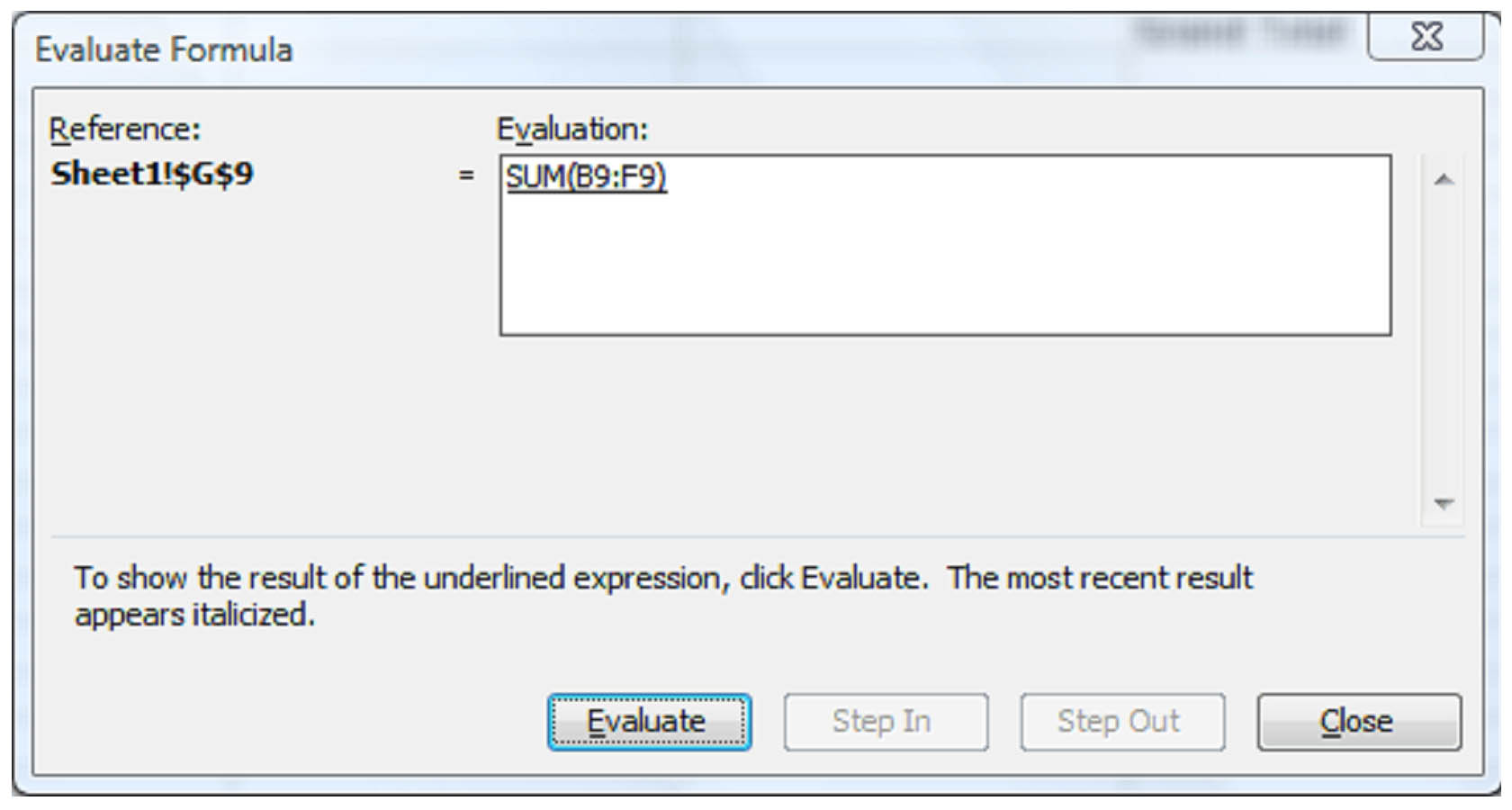
Click the Evaluate button to see Excel perform the calculations in slow motion.  Use the Step In and Step Out buttons to navigate through each step in the formula.