The first step in cutting or copying in Excel is to first select the cells, rows, or columns that you want to cut or copy.
To select a cell, click on the cell. A border appears around it.
To select more than one cell, click your mouse on the first cell you want to select. Ours is A1.
Hold down the left mouse button and drag your mouse until all the cells you want selected are shaded in gray:
Copying Cells
After you've selected the cells or range of cells that you want to copy, you can do one of two things.
- Right click and select.
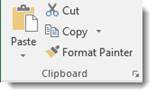
- Go to the Home tab, then select Copy from the Clipboard group.
Copying Rows and Columns
To copy or cut rows or columns, select the number of the row or letter of the column that you want to copy or delete by clicking on the number (row) or letter (column). Remember to click on the number of the row or the letter of the column � not the label.
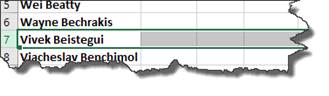
The row selected in the snapshot above is now ready to cut or copy.
Pasting Cells, Rows, and Columns
When you copy cells, you first paste them to the clipboard. Pasting to the clipboard is automatic whenever you select copy, or even cut. The clipboard will hold up to twenty-four different selections so that you do not have to paste right away.
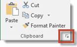
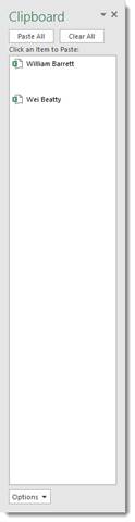
To view the clipboard, click the gray arrow at the bottom right side of the Clipboard group:
All the selections that you have cut or copied will be listed in the Clipboard pane that opens on the left side of the Excel window. See the snapshot below.
If you only want to paste your most recent selection that you copied, all you have to do is go to the place in the spreadsheet where you want to place the copied data. You don't have to mess with viewing all the copied/cut selections on the Clipboard.
To paste your most recent data, select the first cell where you want the data to appear, then go to the Clipboard pane. Right click on the selection you wish to paste, then select Paste.
Paste Special
Excel 2016 gives you a lot of paste options from which to choose. When you go to paste using the Paste tool on the Ribbon or right click on a cell to paste, you can see a half dozen or so little icons appear giving you different ways to paste the data. This can be confusing.
The Paste Special feature makes it a little easier. Paste Special is a dialogue box that allows you to specify how you want to paste the data. Right now, we're still talking about fairly basic Excel features -- and as you start to use Excel yourself -- you'll find Paste Special to be more and more of a help to you.
The Paste Special feature can be found on the Paste dropdown menu under the Home tab in the Clipboard group. It can also be found in the context menu whenever you right click on a cell or a selection of cells.
If you click Paste Special, you will see the following Paste Special dialogue box.
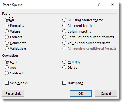
All will paste all the stuff that's in the cell you copied or cut. This includes formatting, formulas, etc.)
Formulas will paste the text, numbers, and formulas in a cell without their formatting.
Values will convert formulas in the current cell to their calculated values upon paste.
Formats will only paste the formatting from the current cell into the pasted cell.
Comments pastes only comments attached to a cell.
Validation pastes only the data validation rules into the cell range set up using the Data Validation command. This will allow you to see values or ranges of cells allows in particular cell or range of cells.
All Using Source Theme pastes all information plus cell styles.
All Except Borders allows to paste everything without the borders used in the source cell.
Column Widths allows you to apply column widths from the copied cell to the pasted.
Formulas and Number Formats allows you to paste the number formats assigned to the pasted values and formulas.
Values and Number Formats converts formulas to their calculated values and includes the number format. The formula will not show up in the Formula Bar in the pasted cell.
All Merging Conditional Formats allows you to paste Conditional Formatting into your cell range.
None will prevent Excel from doing any math between the data entries that you cut/copy and the data entries in the cell where you paste.
Add will add the cut/copied data with the data in the cell where you paste.
Subtract will subtract the cut/copied data from the data in the cell where you paste.
Multiply will do the same as Add/Subtract, except it will multiply.
Divide will divide the copied/cut cells by the data in the pasted cell.
Skip Blanks. Check this box if you want to paste everywhere EXCEPT empty cells in the selected range.
Transpose. Check this box if you want to change the orientation of the pasted entries, such as if you want to change the cells' entries from running down the rows of a single column to running across the columns of a row.
Paste Link is for when you are copying cell entries, and you want to link the pasted entries with the entries you're pasting.
Inserting Rows and Columns
Naturally, there are going to be times when you create a worksheet and then realize that you need another row or column. Since most of the data is already entered, it's too much trouble to use copy and paste to move every column to the right or every row down. Instead, it's easier just to insert a new row or column into the worksheet.
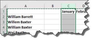
To insert a new column, select the column that comes after where you want the new column to appear. In the example below, we want a new column to appear before the column that is currently �C', so we've selected column �C'.
Next, you can either:
- Right click and select Insert.
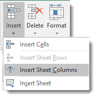
- Go to the Home tab. In the Cells group, click the downward arrow beside Insert. Select Insert Sheet Columns. There will then be a new column where �C' is located in the above picture.
To add a new row, select the entire row by clicking on the row number. Make sure you click on the row number that appears below where you want the new row to be located. The new row will appear above the selected row.
Next:
- Right click and select Insert.
- Go to the Home tab. In the Cells group, click the downward arrow beside Insert. Select Insert Sheet Rows.
Inserting Cells
You can shift cells either down or to the right when you insert a new cell. Select a cell in your worksheet, right click, and select Insert. You will then see the Insert dialogue box.
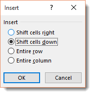
Note: You can also add an entire row or column from this dialogue box.
You can also go to the Home tab, the Cells group, then Insert. Select Insert Cells.
Filling Cells with a Series of Data (AutoFill)
Remember those tests in school where the teacher would make you number a piece of paper from 1 to 10? Have you ever used MS Excel to make a list and put a number in each cell by typing one number at a time, one cell at a time? What about a date?
Typing any type of series in Excel 2016 just takes a matter of minutes if you know what you're doing. You can easily start a series, whether it's a series of numbers, dates, or a built in series for days, weeks, months, and years.
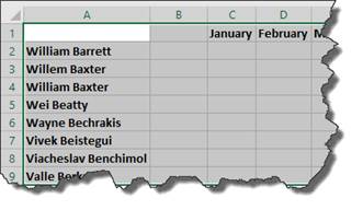
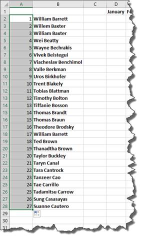
Here's an example. In the screen shot below, we have inserted a column before our employee names. Now, we want to number each employee so we know how many total employees we have.
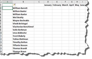
Notice that the cell to the left of the first employee is selected. We will put a number "1" in that cell. However, for the time being, look at the AutoFill handle bar that's closed at the bottom right hand corner of the selected cell.
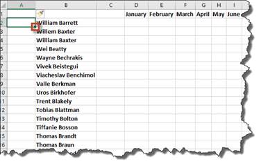
Let's start entering numbers into the cells. We are going to fill in cells A2 through A5 and number the employees.
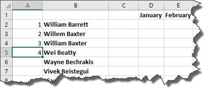
To AutoFill the rest of the series, select the cells that you filled in. We will select A2 through A5. Next, move the mouse over the handle bar for the last cell you selected. A solid black cross (+) will appear. Once that appears, you drag the handle bar over the other cells to complete the series. For our example, we are going to drag it down to the last employee listed in our sheet.
Keep in mind, if you only have one cell selected and not a series of cells as in our example, it will AutoFill the other cells with the same data that appeared in the selected cell. It will not complete the series because a series is not established. You have to establish the series first.
Just to make sure you know how to use AutoFill to complete a series, let's review.
To use AutoFill to complete a series:
1. Start a series.
2. Select the cells in the series.
3. Drag the handle bar over the cells that you want to fill in with a series of data.
4. The series will be filled in for you.
Things to Remember:
- Drag to the right or down to increase or ascend a series of numbers, dates, etc.
- Drag to the left or up for descending numbers, dates, etc.
- Enter at least two numbers, etc. in the series before using AutoFillOnce the series is filled in, you will see an AutoFill options box appear just below the handle bar. You can choose rather to format � or not format � the data in the cells.

Note: Series of numbers or dates do not have to increase by only one. You can have a series that is comprised of even numbers, patterns, odd days of the month, etc.
Flash Fill
The Flash Fill feature was new to Excel 2013. Flash Fill allows you to take part of the data out of one column and enter the same type of data in a new column quickly with just a few keystrokes. The series of entries appear in the new column once Excel figures out the pattern in your original data so it knows what to copy.
Let's see how it works.
In the example below, we have the full names of employees in the first column. In the second and third columns, we want to separate their first and last names into those respective columns.
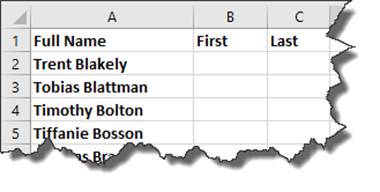
In cell B2, go ahead and type the first name: Trent. When you're finished, hit the downward arrow on your keyboard.
In cell B3, type "t" for Tobias.
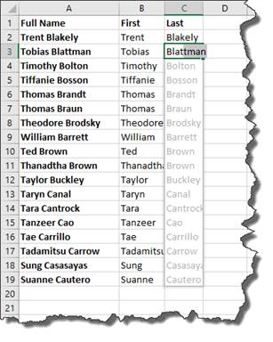
As you can see, Excel detects the pattern in the data and fills in the cells for you.

Click an empty cell in your worksheet.

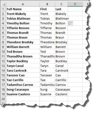
Now repeat the same steps for the last name column.
Click an empty cell.
Multiple Entries
If you have several cells that you want to enter the same data into, you can do this very quickly and easily. Let's say that you want to add the number 43 into seven cells within your spreadsheet. Instead of scrolling through your worksheet and entering it in seven different times, you can do this instead:
- First, select or highlight the range of cells that you want to enter the same data.
- In the active cell, type the data, then press Control and Enter at the same time.
- This will fill in all the cells for you.
Note: If the cells are not adjacent, select the first cell or range of cells, then hold down Control while you select the other cells or range of cells.