How to Graph Algebraic Relations

Key Terms

o Graph

o Real number line

o Real number

o Origin

o Axis

o Coordinate

Objectives

o Understand what the real number line is and how to locate numbers on it

o Be able to construct two-dimensional graphs and find or construct points at specified locations

o Use two-dimensional graphing techniques to plot algebraic relations

An algebraic relation can have a wide range of numbers as "inputs" (the independent variable) as well as a range of numbers as "outputs" (the dependent variable). But looking at a few possible input numbers doesn't always give us a good sense of the general relationship. Even a table of values isn't always the best way to describe the characteristics of the relation. We can, however, use a graph to depict the algebraic relation by showing the value of the dependent variable with respect to the value of the independent variable.

The Real Number Line

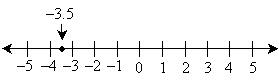
To construct a graph of a relation, we must have an orderly way of listing or showing numbers. The real number line serves this purpose. (The real numbers are the set of numbers that includes the integers along with every possible number between every two consecutive integers. Thus, both rational and irrational numbers are included in the set of real numbers.) The real number line is simply a visual way of showing all the real numbers (within a certain finite range) in order, typically with smaller numbers on the left and larger numbers on the right. Because there are an infinite number of real numbers, we show the number line with arrows on either side to indicate that the actual number line continues indefinitely in both directions. The portion of the real number line between –5 and 5 is shown below. Only the integers in this range are labeled.

Notice that we could extend the line and continue in either direction as far as we wanted. Alternatively, we might focus on a smaller portion of the line, such as between 0 and 1. Because there are an unlimited number of real numbers between any two integers, we cannot label every real number-hence, in the number line above, we only labeled the integers. If we focus on a narrower portion of the real number line, we may wish to label some non-integer values, however.

This and the previous portions of the number line are just two possibilities; what portion of the line we use and which numbers we label depend on the situation. The most important point with the number line is that the numbers be kept in order from smaller to larger. We can show the location of a particular number on the real number line using a small dot. For instance, we can show the location of the number –3.5 as follows:

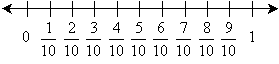
Practice Problem: Draw a number line and plot the point .

Solution: This number is between zero and one, so showing only values between zero and one (inclusive) may be the best approach. The number line below shows the numbers in fifths between zero and one, with identified using a point.

Graphing In Two Dimensions: Two Real Number Lines

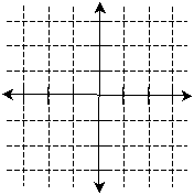
So how can we use the real number line to graph algebraic relations? Such a relation has an independent variable and a dependent variable; a single number line is not much help. If we use two number lines, however, with one dedicated to the independent variable and one dedicated to the dependent variable, we create the ability to graph an algebraic relation. To this end, we use one real number line in the horizontal direction and another in the vertical direction, as shown below. We typically have the real number lines intersect at 0-this point of intersection is called the origin.

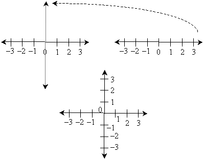
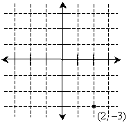
Interested in learning more? Why not take an online Pre-Algebra course?

The use of two number lines in this manner creates a grid, as shown below (the number labels are removed for clarity). Of course, only the grid corresponding to the integer labels is shown-we could show a finer or coarser grid depending on the situation.

Intersection points on the grid correspond to a number on the horizontal axis (or number line) and a number on the vertical axis-these numbers are called coordinates. For instance, we can plot a point corresponding to 2 on the horizontal axis and –3 on the vertical axis. We can express the location of this point as (2, –3), where the first number is the corresponding value on the horizontal axis and the second number is the corresponding value on the vertical axis.

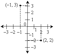
Practice Problem: Draw a two-dimensional graph and plot the points (–1, 3) and (2, –2).

Solution: We can use the same general graph layout that we used in the example above. We omit the gridlines, however, except those that illustrate how to locate the points. Note that the first coordinate in each pair is the number along the horizontal axis, and the second coordinate is the number along the vertical axis.

Graphing Algebraic Relations

We can use our ability to graph points in two dimensions to graph algebraic relations by assigning the independent and dependent variables to the axes of the graph. Typically, the independent variable is shown using the horizontal axis, and the dependent variable is shown using the vertical axis. Conceptually, the approach is simple: for every value of the independent variable (on the horizontal axis), we plot a point whose coordinates are the value of the independent variable and the corresponding value of the dependent variable. Recall that in the previous lesson we evaluated many algebraic relations for particular values of the independent variable and got corresponding values for the dependent variables-we must do the same to plot the relation on a graph.

Of course, we cannot perform this process for every possible value of the independent variable (since there are an unlimited number of these values); thus, we must do out best to pick representative values, which are usually just values chosen at a particular interval. Let's take a simple algebraic relation from the previous lesson and plot it on a graph. We'll only look at a small portion of the possible range of values for the independent variable-in this case, –3 to 3.

In this case, the independent variable is x and the dependent variable is y. Thus, the coordinates of the graph points corresponding to this relation are (x, y)--in other words, for each value of x that we choose, we must evaluate the expression y = x + 1 to get the second (y) coordinate. Let's do this for integers between –3 and 3, inclusive; we'll show the coordinates in a table and then plot them on the graph. We omit the grid lines for clarity.

–3

–2

–1

Several points about the graph above are noteworthy. First, we have only plotted a finite number of points, but the algebraic relation applies to all real number values of x; thus, we must connect the points to show the actual graph. Second, we selected an appropriate range of values for each number line to show the points from the table-the particular range that is appropriate for a given situation depends on such things as what portion of the graph is to be displayed. No choice is necessarily incorrect, but some choices may be better than others. Third, we have labeled each axis with the corresponding variable so that we can clearly see what is being plotted-this is an important point. Let's now show the graph with the points connected (and then removed for clarity).

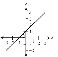
Thus, we see that the algebraic relation y = x + 1 is a line. Let's take a look at another example.

This relation is slightly more complicated, but graphing it requires the same series of steps. This time, we'll omit the table of values, but you can easily verify that the points shown in the graph are correct by considering the x values and the corresponding y values calculated using the relation above. This graph considers x values ranging from –2 to 2.

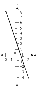
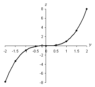
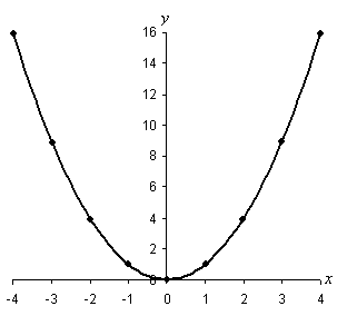
The points in the graph above are also connected, showing that this relation also corresponds to a line. We'll consider one last example--in this case, a relation that does not plot as a line: . We consider x values from –4 to 4, but we don't label every integer on the vertical axis for practicality. Notice also that the graph has points whose coordinates correspond to integer x values, but because they are not in a straight line, we must estimate a curve that fits neatly between the points. To ensure accuracy of the graph, we can simply add more points in between the integer x values--the more points, the better the curve that we draw between them. In the graph below and other graphs in this lesson, we may omit the arrows at either end of the axes, but it is nonetheless assumed that the axes actually continue indefinitely in each direction.

Plotting graphs of other algebraic relations, regardless of their complexity, is very much similar to what we have done for the relatively simple examples above. The following practice problems require that you plot slightly more complicated relations, but if you carefully follow the process discussed above, you should have little difficulty.

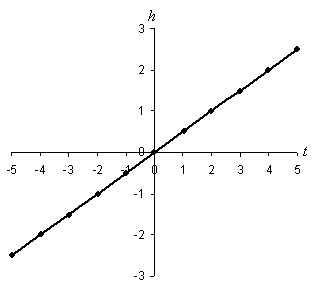
Practice Problem: Plot the relation for t values between –5 and 5, inclusive.

Solution: The plot of this relation is shown below. Note that the independent variable t is shown on the horizontal axis and the dependent variable h is shown on the vertical axis. For each value of t, h is simply half that value. The points on the graph corresponding to integer values of t are also shown.

Practice Problem: Plot the relation for y values between –2 and 2, inclusive.

Solution: We can plot this relation for y values –2, –1.5, –1, –0.5, 0, 0.5, 1, 1.5, and 2, as shown below. The corresponding z value is simply the y value raised to the third power. This relation does not plot as a straight line, so we must draw a curve that fits neatly between consecutive points.