Introduction

 

The techniques for differ from those for linear equations because the inequality signs do not allow us to perform substitution as we do with equations. Nevertheless, we can still solve these problems.

 

Key Terms

 

o         System of linear inequalities

o         Linear optimization

o         Linear programming

 

Objectives

 

o         Learn how to solve problems involving systems of linear inequalities

o         Understand the basic approach to solving linear optimization problems.

 

Systems of Linear Inequalities

 

A system of linear inequalities involves several expressions that, when solved, may yield a range of solutions. Many of the concepts we learned when studying systems of linear equations translate to solving a system of linear inequalities, but the process can be somewhat difficult. Perhaps the most lucid way to simultaneously solve a set of linear inequalities is through the use of graphs. Let's consider an example in two dimensions right away.

 

2x – 5y ≤ 3

y – 3x ≤ 1

 

Because of the inequality, we cannot use substitution in the same way as we did with systems of linear equations. Let's take a look at the graphs of these inequalities. First, we simplify into a form that's easy to plot graphically.

 

2x – 5y ≤ 3         y – 3x ≤ 1

2x ≤ 3 + 5y        y ≤ 3x + 1

5y ≥ 2x – 3

 

Now, we plot the graph of these inequalities.

 

 

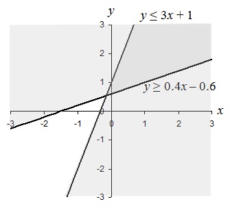
We can see in the graph that there are two shaded regions corresponding to the solutions to each inequality. The lines are shaded because the inequalities are not strict (≥ and ≤ are used). The solution to the system of inequalities is the darker shaded region, which is the overlap of the two individual regions, and the portions of the lines (rays) that border the region. Symbolically, we can perhaps best express the solution in this case as

 

0.4x – 0.6 ≤ y ≤ 3x + 1

 

Solving systems of inequalities in three or more dimensions is possible, but it is much more complicated-graphing the solid regions that constitute the solutions is likewise tougher. 

 

Practice Problem: Find and graph the solution set of the following system of inequalities:

 

x – 5y ≥ 6

3x + 2y > 1

 

Solution: First, let's solve the expressions for y.

 

x – 5y ≥ 6               3x + 2y > 1

x ≥ 6 + 5y               2y > 1 – 3x

5y ≤ x – 6                  y > 0.5 – 1.5x

y ≤ 0.2x – 1.2

 

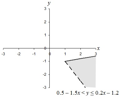
We can then express the solution to this system of inequalities as follows:

 

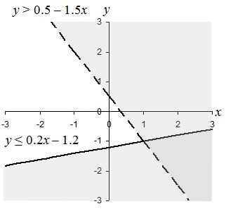
0.5 – 1.5x < y ≤ 0.2x – 1.2

 

Let's graph the solution set. First, we'll graph the lines corresponding to the two individual inequalities (and choosing a solid line for the first and a broken line for the second), then we'll shade the two regions appropriately.

 

 

 

Linear Optimization

 

We can apply what we have learned above to linear optimization (also called linear programming), which is the process of finding a maximum or minimum value for some function under certain conditions (such as linear inequalities). Dealing with problems that involve linear optimization do not require you to learn any new skills; they simply require that you apply what you already know. So, let's move right to a practice problem.

 

 

Practice Problem: Find the maximum value of y given –3x + 2y ≤ 4 and x + y ≤ 1 subject to the condition that x ≥ 0.

 

Solution: What we are given is a system of inequalities for which we must first find a corresponding solution set. Within this solution set, we can then find the maximum value of y. So, we can first apply what we already know: let's rearrange the inequalities into a form that we can easily graph.

 

–3x + 2y ≤ 4         x + y ≤ 1             x ≥ 0

2y ≤ 3x + 4          y ≤ 1 – x

y ≤ 1.5x + 2

 

 

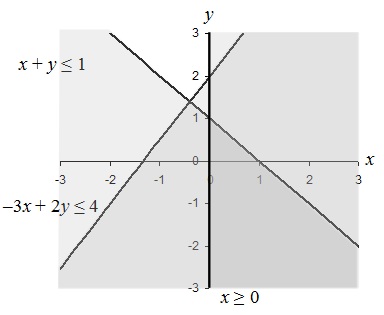
The darkest shaded region (the wedge in the lower right of the graph) satisfies all the constraints on the problem. We then want to find the maximum value of y, which is clearly 1. (We can also find this value by substituting x = 0 into x + y ≤ 1 and finding the maximum value of y, which likewise is clearly 1.)