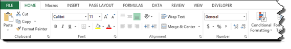
A macro is a series of instructions or commands that can be triggered by a keyboard shortcut, button in the toolbar, or by an icon that you can stick in a worksheet. When you use a macro, you are giving Excel instructions for what you want it to do. However, instead of taking multiple steps to give Excel those instructions, you only take one. Macros are stored in Excel and can be restored to use again and again.
In this article, we're going to explore macros in Excel 2013, including how to:
-
Create and run a macro
-
Save a workbook that contains macros
-
Set the security settings for a workbook with macros
-
Use the personal macro workbook
-
Delete a macro
-
Use absolute or relative references in macros
-
Use a keyboard shortcut to run a macro
Creating and Running Macros
The best way to teach you how to create and run a macro is to walk you through it step by step.
In the worksheet below, we've simply listed the tasks that we want our macro to perform.
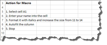
We are going to create a macro that selects sell A1, enters our name into it, makes the font italic and increases the size to 14, then uses autofit to determine the column size.
Notice that #5 is telling the macro to stop. This is important. You record a macro. Just as with anything you record, you must tell it to stop.
Let's create the macro.
To record a macro, you can go to the Developer tab and click Record Macro, or you can go to the bottom of your worksheet and click the button to the right of the word Ready. It looks like this:

You will then see the Record Macro dialogue box.
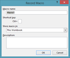
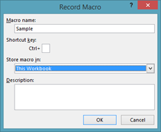
First, give your macro a name in the Macro Name field. You can name your macro anything you want; however, the name cannot contain spaces.
Next, we can tell Excel what keyboard shortcut to use. We aren't going to fill that in right this second. Instead, let's move on to the next field.
In Store Macro In, you have three choices.
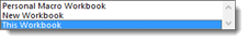
Out of these three choices, there are only two that you need.
-
Personal Macro Workbook stores the macro with your machine.
-
This Workbook stores the macro with your current workbook. If you send the workbook via email to someone else, the macros will be there for them to use.
We are going to choose This Workbook.
Next, enter a description for your macro.
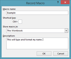
Click OK.
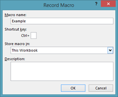
When you click OK, the recorder starts to run.
If you look at the ribbon under the Developer tab, you can see that it says Stop Recording where the Record Macro button was before you clicked it.
To the right of the word Ready, you will see a white square that looks like a Stop button on a tape recorder.
You can click either one of these things to stop recording your macro.
Now, you can start recording your macro by performing the actions we listed.
Take your time when you record your macro. If you make a mistake, even if you undo it, Excel records that mistake. Excel does not record the time it takes for you to enter your macro though. That said, it's important that you take your time.
Record your macro, then press Stop Recording.
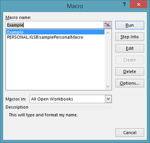
To make sure your macro recorded or to access your macro, go to the Developer tab again. Click the Macros button.
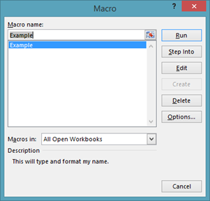
Our macro, Example, is now shown in the list.
If you want to run the macro, click the Run button.
Saving a Workbook with Macros
It's very important when you save a workbook that contains macros, that you save them as macro-enabled workbooks. If you do not save them as macro-enabled workbooks, the macros won't be saved.
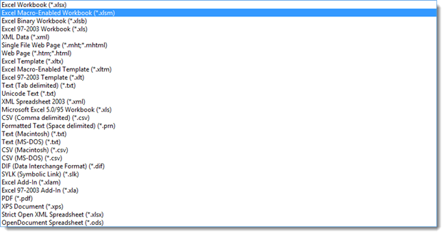
To save a workbook with macros, go to File>Save As.
In Windows 8, choose the location where you want to save the workbook.
In the Save as Dialogue box, go to the Save as Type field and choose Excel Macro-Enabled Workbook, as highlighted in blue below.
Notice that macro-enabled workbooks have a different file extension. It is .xlsm. A workbook without macros is .xlsx.
You can then name your file and click the Save button.
Macro Security Settings
Now that we've saved our macro-enabled workbook, we also need to set the security settings for our workbook since it has macros.
To do this, we will go to the Developer tab again. This time we will click the Macro Security button.
This takes us to the Trust Center and automatically opens it with the Macro Settings tab selected.
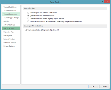
Under Macro settings, you can establish the security settings.
By default, Disable All Macros with Notification is checked. You want to leave this checked. Whenever you open a workbook that contains macros, you will be asked if you want to enable the macros.
Click OK.
When you save and close a workbook, then reopen it, you will see this message above your worksheet.
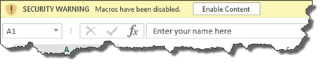
Click the Enable Content button so that you can use the macros in the workbook.
Once you enable the content for a workbook, you will not see the security warning again for that workbook. The content will automatically be enabled.
The Personal Macro Workbook
The personal macro workbook doesn't exist until you create it. You create a personal macro workbook when you create and save your first workbook, choosing to save it to your personal macro workbook. Each time you open Excel, the macros you created in your personal macro workbook will be there for you to use. Your personal macro workbook will be available to you no matter what Excel workbook you open � as long as you open it on the machine where you created the personal macro workbook.
For example, if you create the personal macro workbook on your desktop computer that you have at home, the macros that you save to that personal macro workbook will be available to you. It doesn't matter what workbook you created them in. They will be available in all workbooks that you open while on your home desktop computer.
However, if you use your laptop or a computer at the office, the personal macro workbook, as well as the macros, that you created on your desktop computer will not be available to you. Your personal macro workbook and all the macros included in it are machine specific.
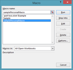
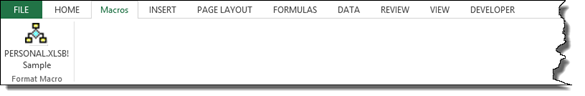
That said, when you open your macros, you will be able to distinguish macros that are part of your personal macro workbook from macros that are workbook specific. The macros that are part of your personal macro workbook will have PERSONAL.XLSB! in front of the macro name, as shown below.
To create and store a macro in a personal macro workbook, click Record Macro under the Developer tab.
In the Store Macro In field, select Personal Macro Workbook from the dropdown menu.
When you store a macro in your personal macro workbook, Excel will confirm that you want to save that macro in your personal macro workbook when you try to exit Excel. This only happens the first time you exit Excel after storing a macro in your personal macro workbook.
You will see the message shown in the screenshot below.
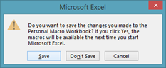
If you click Save, the macro is saved to your personal macro workbook.
If you click Don't Save, then the macro will not be saved and will not be available in any workbook again.
NOTE: If you like to back up your files, the file that contains your personal macro workbook is titled XLSSTART. The path to it will always be Microsoft>Excel>XLSSTART. Where your Microsoft folder is stored will depend on your operating system and installation.
Deleting a Macro
To delete a macro that you have saved to a workbook, go to the Developer tab, then click on the Macros button.
Select the macro by clicking on it, then click Delete.

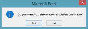
You will then see this message:
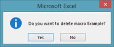
Click on the Yes button if you want to delete the macro.
If you try to delete a macro that's included in your personal macro workbook using the steps we just detailed, you will see this message:
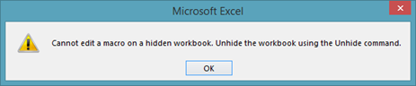
It tells you to unhide the workbook before you can delete it. Click OK.
We will show you how to unhide the workbook in a minute. For now, it's important to remember that macros stored in your personal macro workbook are stored in the PERSONAL.XLSB workbook. When you open another workbook in Excel, those workbooks are available to you to use. However, the macros aren't stored in the workbook you've opened. Again, they are stored in the PERSONAL.XLSB workbook instead.
In order to delete a macro from the PERONSAL.XLSB workbook, you must first unhide it.
To unhide the workbook, go to the View tab.
Click Unhide in the Window group.
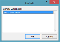
Select the workbook you want to unhide. You can see that our personal macro workbook is listed.
Click OK.
The personal macro workbook is now open on your machine. To delete a macro from it, go to the Developer tab.
Click the Macros button.
Select the macro that you want to delete, then push the Delete button.
You will see this message:
Click Yes.
Close your personal macro workbook as you would any other workbook.
You will then see this message:
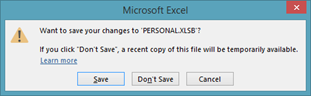
Click Save to save the changes.
The Use of Relative or Absolute Referencing in Macros
Remember, an absolute cell reference is when you want a cell reference to be fixed on a cell. In Excel, you can mark rows and columns as absolute by adding the dollar sign ($) before either the row, column, or both when working with formulas.
A relative cell reference is a cell reference that can change when something, such as a formula, is copied from one cell to another.
In Excel 2013, whenever you create and record a macro, the cell references are automatically absolute. If you create a macro that starts in A1, if you use that macro in a different worksheet, it will start in cell A1. It doesn't matter which cell is active when you run the macro, it will run in cell A1.
When you create an absolute reference when recording a macro, you can have the macro run in any cell. For example, you can create the macro while cell A1 is active. When you run the macro, you can run it with cell F4 active, and the macro will run in cell F4.
To use a relative reference when recording a macro, go to the Developer tab, then click the Use Relative References button.
Next, click the Record Macros button.
Go ahead and name the macro, then choose where you want to store it. You can also enter a description.
Click OK.
When you're finished, stop recording.
Now you can click on any cell in a worksheet, go to macros under the Developer tab, then run your macro. It will appear in the cell that's active.
If you don't want future macros to have relative references, make sure you go back to the Developer tab and click Use Relative References again to turn off the use of relative references when recording macros.
Using Keyboard Shortcuts to Run Macros
Thus far in this article, whenever we wanted to run a macro, we went to the Developer tab, then clicked the macros button. However, since macros are supposed to save time and create shortcuts, this can seem like extra work that's not really needed.
Instead of going to the Developer tab and clicking Macros every time you want to run one, you can instead assign a macro a keyboard shortcut. The keyboard shortcut always involves the CTRL key, plus a letter on your keyboard. You must choose a letter. Your shortcut cannot involve numbers or symbols.
If you choose an uppercase letter, the keyboard shortcut will be CTRL+Shift+ the letter that you choose. If you choose a lower case, it will simply be the CTRL key plus the letter that you choose.
Let's create a new macro by going to the Developer tab, then clicking Record Macro.
Go ahead and name the macro.
Enter the shortcut, as we've done below.
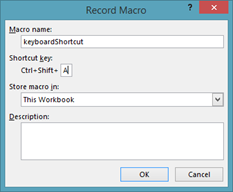
When you're finished, click OK, the record your macro.
Stop recording when you're finished.
What we learned in the last section about macros was just the tip of the iceberg. We are going to continue to explore macros in this section and learn more about creating and working with them.
We will talk about how to:
-
Apply formatting using a macro
-
Switch between scenarios using a macro
-
Switch between custom views using a macro
-
Using worksheet buttons to trigger macros
-
Customizing buttons and other shapes that trigger macros
-
Adding macros to the ribbon
-
Creating your own ribbon
-
Adding a confirmation box to a macro
Formatting with Macros
Formatting cells in workbooks can be a tedious process, especially if you have to format each worksheet in workbooks that you create. To save time and make things easier, you can use macros to format cells and worksheets simply by creating macros that do all the formatting for you. This way, you only apply the formatting once. After that, all you have to do is run the macro.
A macro can contain as many steps as you want it to contain. You can create a macro that changes the font type, color, and size, then also applies cell formatting and row and column sizes. In essence, you can create macros to do all the formatting for you.
We are going to create a macro that does the following things:
1. Changes font type, size, and color.
2. Sets a theme (under the Page Layout tab).
3. Formats the cells to Number with three decimal places.
4. Creates a table in the worksheet.
We are going to call this macro salesWorksheetFormatting.
Notice that we are storing this macro in our personal macro workbook. This way, it's available in all workbooks, and we can use it no matter what workbook we have open.
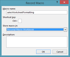
Click OK.
We can then record our macro.
Remember to stop recording when you finish all the steps involved in your macro.
Switching Between Scenarios with Macros
If we go to the Data tab, then click the What-If Analysis button, then click on the Scenario Manager, we can see all the scenarios we've created.
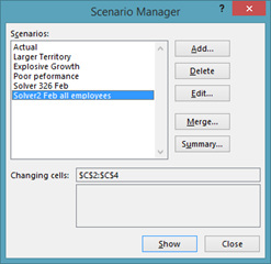
We can select any of these scenarios, then click Show to see the scenario in our worksheet.
If we want to see another scenario, we go back to the Scenario Manager, select the scenario we want to view, then click the Show button again.
This is a lot of clicks.
Instead, we can create a macro for each scenario and add a keyboard shortcut for each macro that we create. That way, we can view a scenario simply by using a keyboard shortcut.
To create a macro for a scenario, go to the Developer tab and select Record Macro.
Name the macro so that you know which scenario it is, then specify a keyboard shortcut.
You will want to store the macro in the workbook.
Click OK, then record yourself opening up the Scenario Manager, selecting a scenario, then clicking the Show button.
Stop recording when you are finished.
You can now view that scenario by running the macro.
Switching Between Custom Views with Macros
In addition to creating macros to view scenarios, you can also create macros to access custom views.
Go to the View tab and select Custom Views.
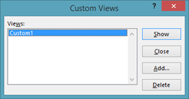
Select a custom view.
If you click the Show button, the custom view will appear in the worksheet.
Instead of having to click the View tab, click the Custom Views button, then click the Show button, you can instead create a macro with a keyboard shortcut that will do all of this for you.
To create the macro, click the Record Macro button under the Developer tab. Name the macro, then assign a keyboard shortcut to it. You will want to store the macro in the workbook.
Click OK, then record yourself going to the View tab, clicking the Custom Views button, then clicking the Show button.
Remember to stop recording when you are finished.
You can now switch to that custom view by simply running the macro.
Using Worksheet Buttons to Trigger Macros
In the last section, we learned how to create keyboard shortcuts to trigger macros. That said, the problem with creating keyboard shortcuts to trigger macros is that, if you have a lot of macros, it can be hard to remember what keyboard shortcut triggers what macro.
Imagine having twenty macros for one workbook, then trying to remember which macro triggers cell formatting. It can be impossible and actually make things more complicated. Macros are supposed to make things easier.
Instead of creating keyboard shortcuts, you can create worksheet buttons instead.
A worksheet button is just as it sounds. It's a button that you place in your worksheet. When you click on that button, it triggers a macro.
To create a worksheet button that will trigger a macro, click in the worksheet where you want to place the button.
Go to the Developer tab. Click the Insert dropdown arrow.
The first icon in the top left corner is a button. Click on the button icon.
Your mouse cursor now is a crosshair.
Click and drag to draw the button.
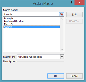
When you release your mouse, you will see the Assign Macro dialogue box.
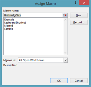
Click on the macro that you want to assign to the button.
Click OK.
The button then appears in the worksheet.
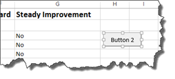
Now you can rename the button. It's recommended that you give the button the same name as the macro or a name that will remind you what the macro actually does.
You can also drag on the button handles to resize it.
When you're finished, click in the worksheet.
The button is now clickable.
Now, whenever you click on the button, it will run the macro.
Customizing Buttons and Other Shape Triggers
You can apply some customization to worksheet buttons and other shape triggers.
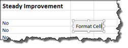
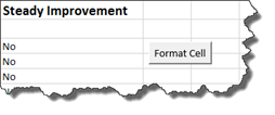
To apply customization, select the button. To do this, you will have to right click on it. If you just left click on it, it will run the macro. Instead, right click on it, then select one of the options in the context menu.
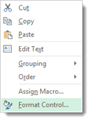
We are going to select Format Control.
This brings up the Format Control dialogue box.

You can click through the tabs to apply different formatting options to your button.
-
The Font tab gives you options to format the text on your button.
-
The Size tab allows you to change the size of the button.
-
The Alignment tab allows you to align the text on the button.
-
The Protection tab allows you to lock an item or lock the text.
-
The Properties tab allows you to control the positioning of the button.
-
The Margins tab allows you to set margins inside the button.
-
The Alt Text tab shows you the label for the button.
Apply any formatting that you want using this dialogue box, then click OK when you're finished.
If you noticed, the one thing you couldn't change was the color of the button. When we go to the Developer tab to insert a button, we are left with very few formatting choices. For example, grey is the only color of button we can insert, and it's always going to be either a square or rectangle shape.
If we want to use buttons that have different colors and styles � or even use other shapes as buttons, we need to first create a shape and format it.
Click the Insert tab, then go to Shapes. Select the shape that you want to use, then drag to draw it on your worksheet as we've done below.
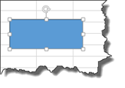
We have chosen to use a rectangle. However, you can use any shape. It does not have to be a rectangle.
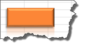
The Drawing Tools Format tab is now open on the Ribbon.

Apply a shape style to the shape if you want. You can also change the shape fill and outline colors. In addition, you can add effects such as a drop shadow.
Our shape is shown below.
Next, right click on the shape and choose Assign Macro.
Select the macro that you want to assign to the shape, then click OK.
That macro is then assigned to the button. Whenever you click the button, the macro will be triggered.
Now, right click on the button and choose Edit Text. Add a text label to the button so you know which macro will be triggered when you click on it.
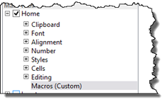
Assign a Macro to a Ribbon Icon
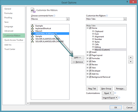
You can also add buttons to the ribbon that will trigger macros. To do this, first go to File>Options.
Click the Customize Ribbon tab.
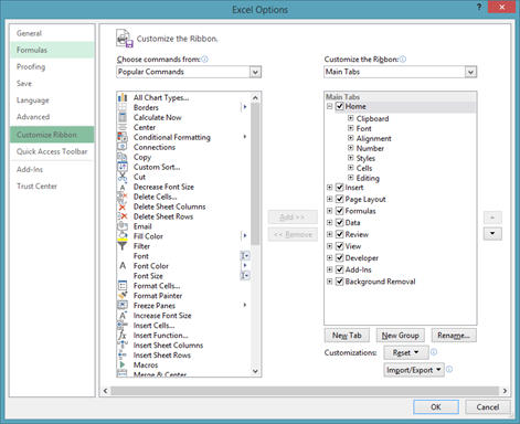
From the Choose Commands From dropdown menu (where it currently says Popular Commands), choose Macros.
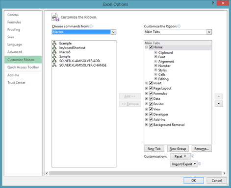
You can now see your macros.
Go to the Customize the Ribbon section. Choose the tab where you want to place your macros by clicking on it. Do not uncheck the other tabs. This will cause them to not appear on your ribbon.
We are going to choose the Home tab.
Now, you also have to select the group. However, you can't place the button in an existing group. Instead, you have to click the New Group button, as pictured above.
You will then see New Group (Custom), as highlighted in grey above.
Next, click the Rename button that appears to the right of the New Group button.
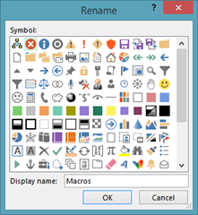
Rename the group. We are naming ours Macros.
Click OK.
Now, select the macro that you want to add to the group. You will select it from the field on the left, then click the Add button that is between the two fields.
Click the Rename button again.
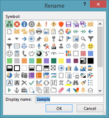
Click on a symbol to represent the macro. You can also rename it if you want.
Click OK.
When you've added all your macros and selected symbols, you can click OK to leave the Excel Options dialogue box.
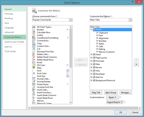
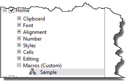
Take a look at our Home tab. You can see our new Macros group to the far right on the ribbon.

NOTE: Typically, you will want to use macros that are stored in your personal macro workbook for this. That way, whenever you open Excel, those macros are on your ribbon and available to you.
Creating Your Own Ribbon
In addition to adding macros to an existing tab, such as Home as we did in the last section, you can also create your own tab just for your macros.
To do this, go back to File>Options>Customize Ribbon.
Click New Tab, as shown below.
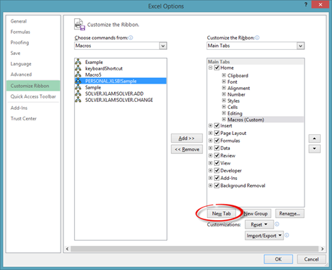
Our new tab is then visible.
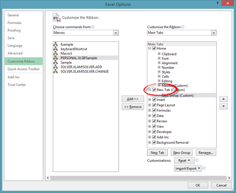
Click the Rename button, as we did in the last section.
Name your new tab, then click OK.
Now you can name the group that's included in the tab by default. Right now, its name is New Group.
You can also add more groups by clicking the New Group button.
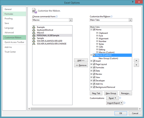
Next, add macros to the group.
When you're finished, click OK.
You can then see the Macros tab in the ribbon.
If we click on the Macros tab, we can see our group.
Editing Macro Code
It's not recommended that you ever attempt to edit the Visual Basic code for your macros. However, just in case you ever need to, we will show you the basics that you need to know in order to be able to make minor changes.
Just be warned, anything outside of the basic editing that we will teach you is a task best left for experienced programmers and not for the typical Excel user. If you mess up the code, you will require the assistance of a programmer to fix it, or you will have to re-record the macro.
To view and edit macro code, go to the Developer tab and click the Macros button.
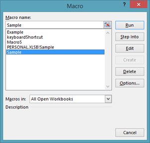
Select the macro that you want to view and edit, then click the Edit button.
NOTE: If you are going to edit code in a macro that's stored in your personal macro workbook, you will need to unhide the workbook first.
Once you click the Edit button, this is what you will see:
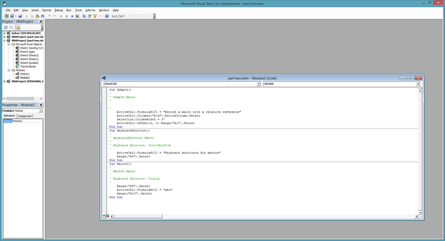
The macro code is shown below.
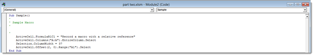
At the top you see Sub Sample. Sub is for subrooting. Then you see the name of your macro.
At the end you can see that the subrooting is ended. It says End Sub.
Everything in between Sub and End Sub are instructions that the macro will carry out.
Any line where you see an apostrophe at the beginning, followed by green text, are comments. They are not actionable code. You can add more comments if you want. This is very basic, and you're not going to hurt anything by doing this.
Now let's look at the actual code, which is anything in black font that's between Sub and End Sub.

You will see that some of the code appears between quotation marks, such as "Record a macro with a relative reference." This is actually the text that appears in our worksheet when we run the macro. If you want, you can edit text that appears between quotation marks. Again, this is easy enough, and you don't do any damage.
Other things that may appear in your macro that you can easily change are:
-
Font type . Just type in a new font type, such as Arial.
-
Font size . Enter a new font size, such as 14.
-
True/False arguments . You can change an argument from True to False, then vice versa.
-
Range . If the range is .Range("A1"), you could change it to another cell, such as A2.
-
Active Cell . Right now, the active cell appears as ActiveCell.FormulaR1C1. R1C1 stands for row one column one. You could change this to R2C2, for example.
If you recognize anything else and feel comfortable changing it, then you can try to do it. Just remember that you may damage the macro in the process and be forced to re-record it.
When you're finished, simply X out of the window by clicking the X in the top right corner. You do not need to do anything to save the changes. You can then run the macro whenever you want.
Adding a Confirmation Box to a Macro
Although it's not advisable that you attempt to edit the code for your macros, there is a circumstance when you will be required to edit that code. If you want to add a confirmation box to a macro, you will have to edit the code in order to create that box.
A confirmation box is a box that will ask you if you are sure that you want to run a specified macro. This is especially helpful to have if you create a macro that deletes cells or data.
Let's show you how to do this.
Go to the Developer tab and click on the Macros button.
Select a macro for which you want to create a confirmation box, then click the Edit button.
You will then see your code.

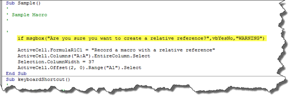
To create the confirmation box, we need to start out by adding an If statement. Click at the beginning of the first line of code. Push the spacebar a few times. Then, click to put the cursor above the first line of code. The next snapshot will show you what we mean.
Once you've done that, we can start to enter the code.
The first thing we type is "if" then add a space, then type "msgbox" to create the confirmation box.
Add an opening bracket, as shown below. We are then told what we need to enter next, as shown below.
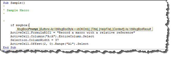
The first thing to enter is a prompt. This is the text that a user will see in the confirmation box that asks them a question.
Type in that question. Any text that will appear inside the confirmation box goes in quotes.
We have customized our prompt to our macro, but your prompt can be anything you need it to be.
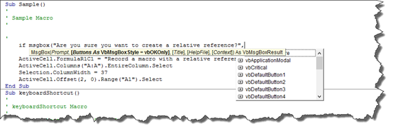
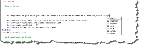
Next, select the buttons. We want Yes and No, so we scroll down in the button dropdown menu.
Double click on the button you want to add. It will appear in your IF statement. Add a comma after it.
Next, you can add an optional title to your dialogue box. We are going to enter "Warning."
You do not need the rest of the parameters for a confirmation box.
Add a closing bracket to your IF statement.
We highlighted our IF statement in the snapshot below.
Next, add an equal sign after your closing bracket.
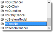
You will see another dropdown menu.
Double click on VBYes in the dropdown menu. This lets Excel know to display the confirmation box. If the answer clicked on in the confirmation box is YES, then to run the macro.
Add a space, then type "then."
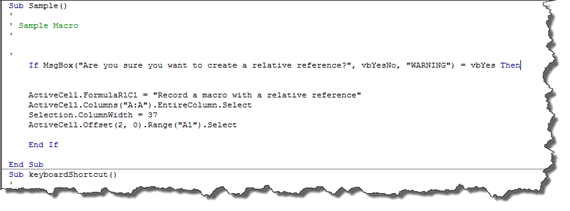
Press Enter.
Next, at the end of your macro, but before the End Sub, type "End If" as we have done above.
Press Enter.
You can now X out of the code window.
Go ahead and run the macro for which you created the confirmation box.
You will see the confirmation box appear on your screen.
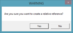
We are going to click Yes.
When you click Yes, the macro runs.