Whenever you save an Excel file to your computer or save it using any other method, it's saved as a workbook. A workbook is made up of worksheets. In other words, worksheets are stored in workbooks, and workbooks are the files that you actually save.
Whenever you open a blank workbook, there is one worksheet created in it by default. In this lesson, we'll learn all about worksheets and workbooks.
Opening Worksheets and Workbooks
When you open a new or existing MS Excel 2016 file from your computer, you are opening a workbook. A saved workbook file looks like this on your computer:

When you open a workbook, you see the first worksheet contained within the workbook.
Any other worksheets within the workbook will appear as tabs at the bottom left corner of the Excel window.
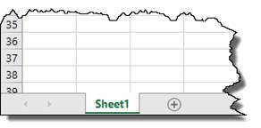
Click on the tab to open the worksheet.
Opening an Existing Workbook
If you want to open an existing workbook, you can do one of two things. You can find the file on your computer, then double click to open it.
If Excel is already open on your computer, go to the Backstage area by clicking the File tab. Click Open on the left.
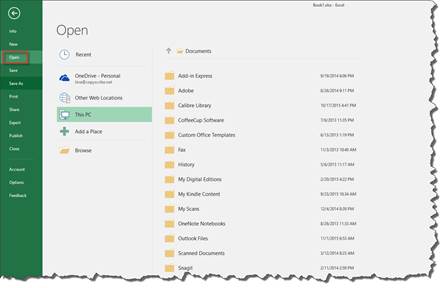
You can then search through recent workbooks, your SkyDrive, other locations on the web, your computer, or you can also add a place you want Excel to look.
Saving a Workbook
It can be argued that the most important thing you need to learn to do in Excel 2016 is to save your workbooks. After all, saving your workbooks is the only way to insure that you won't lose any of your data � and that you can come back to work on it again later.
Let's say that you've created a new workbook and wish to save it on your computer. You can do this quickly and easily in Excel 2016. Click File, then choose either Save or Save As on the left in the Backstage area.
- Clicking Save will enable you to save the file under its current name and keep it saved at its current location. Keep in mind that if this is a new workbook, it will save the file by the default name of Book1. When you click Save, if another file of the same name exists, Excel will prompt you to either enter a new file name or to replace the existing copy with the new version you are currently saving. If you want to save the file to a new location, you must choose Save As.
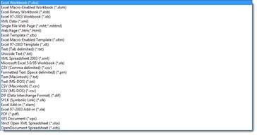
- Clicking Save As gives you a lot more options to saving your work. First of all, when you click Save As, you must specify a file name. You must also specify the format that you want to save the file in. Word's default file format is .xlsx. This is an acceptable and much-used format that should be satisfactory for most Excel users, but you can select the format that you need depending on the work you need to save. Let's show you what we mean.
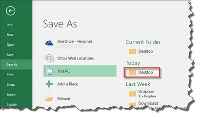
Click File, then choose Save As on the left.
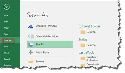
In the "Save As" column, choose where you want to save the workbook. You can save it to your OneDrive, which is your cloud storage. In addition, you can save it to other web locations, This PC � which is your computer -- or you can add a location by clicking "Add a Place".
Let's click on This PC.
Choose the location on your computer where you want to save the file. You can also click Browse to find a location. We're going to choose Desktop.
Enter a name for the file in the File Name text field, as pictured below.
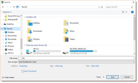
In the Save as Type field, choose the format in which you want to save the workbook.
NOTE: You can also save a workbook by clicking the picture of the floppy disk in the Quick Access Toolbar. This will save the file under the current name in its current location. It's a good idea to click this button every so often while working in a workbook to save it in case of a power outage, computer freeze, or anything else that may cause you to lose your work
Viewing Previous Versions of a Workbook
If you have SharePoint or OneDrive for Business, Excel 2016 saves versions of your workbooks files as you have them open and are working on them. To view the historical versions of your workbook, go to the File tab and click History on the left.
You will see the older versions of the workbook in the History pane.
Click a version to view it in a separate window.
If you want to restore your workbook to that version, click the Restore button in the message bar at the top of your workbook.

About Sheet Tabs
As stated earlier in this lesson, each new workbook that you open in Excel 2016 has one worksheet created for you by default. You can add worksheets to a workbook. You can also delete sheets from a workbook.
By default, the first worksheet contained within a notebook is named "Sheet1". The second worksheet would be "Sheet2", and so on.
However, as you use Excel to create your own spreadsheets, you'll want to rename the worksheets to represent the type of data they contain.
Let's rename Sheet1, for this example.
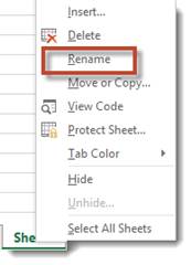
The easiest way to rename a sheet is to move your cursor over the sheet you want to rename, then right click on it with your mouse.
Select Rename from the context menu.
The sheet that you want to rename will then be highlighted, as shown below.
Type the new name. When you're finished, click elsewhere in the worksheet area.
Adding Worksheets
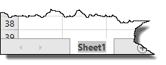
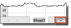
To add a worksheet, go to the Sheet Tabs. Click the plus sign (+) that's to the right of the last worksheet, as shown below.
Here are some things to remember when adding worksheets:
-
Click the sheet tab that will come BEFORE your new sheet tab/worksheet.
-
For example, if you want to put a new worksheet/sheet tab after worksheet two, click Sheet2, then click the plus sign.
Excel then adds the new worksheet under Excel's default name. Once you've created the worksheet, you can then rename it.
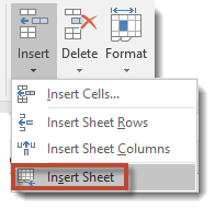
Note: You can also go to the Home tab on the ribbon. Go to the Cells group and click Insert, then select Insert Sheet.
Deleting Worksheets
To delete a worksheet, go to the Sheet Tabs. Select the worksheet that you want to delete, right click, and select Delete.
Hiding Worksheets
Hiding a worksheet allows you to remove it from view of others or simply get it out of your way. When you hide a worksheet, you or anyone else accessing the file will not be able to see it. There will not be a Sheet Tab for it. You'll have to unhide it to be able to view it again.
To hide a worksheet, select the worksheet you want to hide by clicking on its tab.
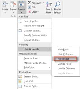
Next, click on the Home tab and go to the Cells group. Click Format.
Select Hide and Unhide from the Visibility group in the dropdown menu, then Hide Sheet.
Unhide a Worksheet
To unhide a worksheet so that you may view it again, follow the same steps as you took to hide the worksheet, except this time select Unhide Sheet.
Hiding Columns
You can also hide data by hiding cells, rows, and columns within a worksheet. There are a few reasons you may choose to do this. It may be to simplify the worksheet and make it easier to navigate or to protect certain information.
As with all Microsoft products, there is more than one way to do a certain task. You can use the steps above for hiding sheets to hide columns and rows. But there's also another way. Let's learn how to hide columns by using the Column Header Bar. This is the bar where the column letters are: A, B, C, etc.
Remember, when you hide a column, data in that column can still be used in the worksheet.
To hide a column:
Right click on the column header of the column that you want hidden. We're going to use column A in this example.
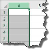
When you right click on the column header (A), the entire column will be selected, as show above. You will also see the context menu. Select Hide from this context menu.
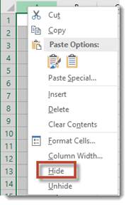
NOTE: If you don't see the context menu, simply right click again, then select Hide.
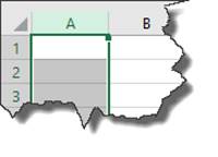
To unhide the column, follow the exact same steps and, instead, select Unhide.
Hiding Adjacent Columns
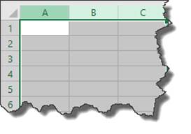
You can also hide more than one column at a time. Let's say, for example, that we want to hide columns A, B, and C. The first thing we're going to do is select column A by left clicking the mouse on the column A header.
Keeping the left mouse button pressed down we're going to drag it over columns B and C to select them as well. See the screenshot below.
When the columns are highlighted, right click the mouse and select Hide. This will hide all three columns.
Hiding Non-Adjacent Columns
If you want to hide more than one column, but the columns aren't adjacent, there's an easy way to do it. Simply click on the first column to be hidden. Press and hold down the Ctrl key on your keyboard while you left click on the other columns to be hidden. Now, right click on one of the columns that you selected and choose Hide from the menu. This will hide all the selected columns.
Hiding Rows
You can easily hide rows in MS Excel 2016 in the exact same way that you hide columns. The only difference is that you're going to click on the number of the row that you want to hide. This selected the entire row. Next, right click your mouse and select Hide.
Note: Remember, to unhide a row, you follow the exact same steps, but select Unhide instead.