Key Terms

 

o       Regression analysis

o       Linear regression

o       Method of least squares

o       Least-squares linear regression

o       Covariance

o       Correlation

o       Correlation coefficient

 

Objectives

 

o       Understand the basic foundation of regression (specifically, least-squares linear regression)

o       Recognize the correlation coefficient and what it measures

o       Derive and simplify simple expressions for the correlation coefficient and the regression parameters

o       Perform a linear regression for a data set

 

In regression analysis, we will fit an algebraic function to data. Although data can follow a number of different trends, such as linear, exponential, polynomial, and logarithmic, we will focus exclusively on linear regression, which is the simplest type of regression analysis. Linear regression attempts to determine a linear function (that is, a line) that best describes the trend of the data. Of course, any data set can be fitted to a line, but not all data sets can be fitted accurately to a line. Thus, we will also discuss how to quantify the "goodness of fit" for a linear regression.

 

Method of Least Squares

 

Perhaps the most common form of linear regression uses the method of least squares; this approach attempts to minimize the sum of the squared distances between the data points and the regression line. The use of this method in linear regression is often called least-squares linear regression. Although a complete derivation of the formulas used in this method requires an understanding of differential calculus, we can present a sufficient outline of the approach to this problem as follows.

 

Consider a data set {{x₁, y₁}, {x₁, y₁}, {x₁, y₁},., {x_n, y_n}}. We want to find a line that best describes the data-to do so, we will attempt to minimize the sum of the squared distances between the line and the data points (we square the distances to avoid cancellation due to sign variations). Let's define our regression line as y = mx + b, where m is the slope of the line and b is the y-intercept of the line. Also, let's define the distance between a point and the line as the vertical distance-we make this choice because we are determining the distance for a given value of x (one which corresponds to the x value of the point in question). Then, given any point (x_i, y_i), the distance d_i between the point and the line is

 

d_i = y – y_i = mx_i + b – y_i

 

Note that if we know m and b, then we know the distance d_i. The sum of the squared distances is then

 

 

The scatterplot and (solid) regression line below illustrates the (dashed) distances used for least squares.

 

 

Using differential calculus, we can use the preceding expressions to calculate m and b. (This exercise is left to you, should you already be familiar with differential calculus.) Instead of going through all of the extensive mathematical gymnastics needed to derive expressions for m and b, we will simply write the results below.

 

  

 

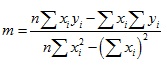
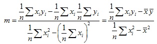
(Each summation above is from i = 1 to i = n.) Note that we can express these formulas in terms of the means of x and y, which are and , respectively. (We use Latin letters since the data will typically be a sample of a population.)

 

 

The formula for b is simple enough once we calculate m. But we can further simplify m by noting the relationship of the denominator to the sample variance of x, . Let's prove this statement starting with out definition of the sample variance.

 

 

Also, we can relate the numerator of m to the (sample) covariance of x and y, s_xy, which we define as

 

 

The covariance is actually a measure of correlation between the random variables (a subject that we will discuss further later), and it can be either a positive or negative value (–∞ ≤ s_xy ≤ ∞).

 

Then,

 

 

Combining these results gives us

 

 

So, we can calculate m and b using just , , , and . Note that although we have written the coefficient m in terms of sample statistics, the regression formulas apply to populations and to samples--our original definitions of m and b apply regardless of the type of data used.

 

 

Practice Problem: Find the line that best fits (in the least-squares sense) the following data set:

 

{(12.0, 9), (10.1, 19), (21.2, 29), (20.4, 39), (34.9, 49), (38.3, 59), (40.2, 69),
(40.5, 79), (51.6, 89), (53.5, 99)}

 

Solution: When performing a regression, sketching a scatterplot is helpful both to visualize the data and to get a sense of where the regression line will lie. Once we perform the regression, we can also plot the line to see if it looks correct--if the line doesn't seem to fit the data, then we know to check our calculations (or our plot) for a possible error. Below is a scatterplot for the data provided in the problem.

 

 

To determine the line that best fits the data (using least-squares linear regression), we need to calculate several parameters for the data. Let's start with the means for the x data (the first value in each pair) and the y data (the second value in each pair). Note that the data set contains 10 total pairs.

 

 

Next, let's calculate the covariance, , and the variance of the x data, .

 

 

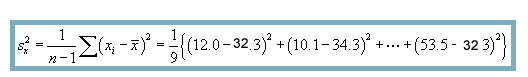
Using the values we calculated above, we can now determine the regression parameters m and b, which are (respectively) the slope and intercept of the regression line for this data.

 

 

The regression line is thus y_i = 1.90x_i – 7.37. Let's check the result by overlaying the line on the scatterplot. Note that we limit the line so that it only covers the area in which the data is located (that is, the domain of x values)--we don't know anything about the possible behavior of the population (if it exists) beyond these limits, because such data is not provided.

 

 

From the plot above, we can tell that the regression produced a result that closely aligns with the provided data. Although this does not prove, by itself, that we have done all our calculations correctly, it does increase our confidence in those calculations.

 

 

Correlation Coefficient

 

We can also produce a numerical value for how well a set of data fits with a regression line. This value can be viewed as a "goodness of fit" measurement, which expresses the linear correlation of the data for two random variables. The correlation coefficient r is

 

 

As with the regression coefficients m and b, we can also simplify this into some known statistical values:

 

 

Thus, the correlation coefficient can be expressed in terms of the covariance, s_xy, and the standard deviations s_x and s_y. The correlation coefficient ranges as –1 ≤ r ≤ 1, where a larger magnitude indicates more linear character (correlation) and a smaller magnitude indicates less linear character. A positive sign indicates that the slope of the linear relationship is positive, whereas a negative sign indicates that the slope of the relationship is negative.

Practice Problem: Determine, using a quantitative justification, whether the following data has enough of a linear relationship to warrant linear regression.

 

{(3, 23.9), (4, 81.6), (7, 35.4), (9, 31.5), (14, 69.9), (16, –21.4), (19, –4.2), (20, 49.6), (22, 37.7)}

 

Solution: We can decide whether the above data warrants linear regression by calculating the correlation coefficient, r. First, let's get a qualitative picture by sketching a scatterplot of the data.

 

 

Based on the arrangement of the data points, no clear linear relationship is indicated. Thus, we should expect to calculate a relatively low value for r. To do so, we must first calculate the means of the x and y data.

 

 

Next, we must calculate the covariance s_xy and the standard deviations s_x and s_y.

 

 

 

 

 

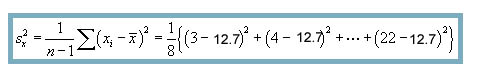
Finally, let's calculate the correlation coefficient.

 

 

Note that this correlation coefficient is indeed small, and thus, the data is not sufficiently correlated to warrant performance of a linear regression. (The exact range of r values for which regression is warranted is, of course, somewhat subjective. In this case, the value is quite small, and the scatterplot shows no linear trend, so we conclude that the data does not demonstrate much linear correlation.)