The ability to use formulas and perform calculations is the bread and butter of MS Excel.
Of course, if you're anything like me, your palms just got sweaty at the mere mention of the words ‘formula' and ‘calculation.' You remember all of those late night cram sessions in high school or college, the creased brow, the books that didn't illuminate anything, the bad feeling that maybe you were in way over your head. On those nights you'd just say to yourself, ‘do I really need to know any of this? It's not like I want to be a mathematician or anything!'
If that was your reaction to math too, you can relax. You do not have to be a math wiz to understand or use these functions in MS Excel. In fact, if you were a math wiz, you probably wouldn't even need Excel.
Definition and explanation of formulas and calculations
In Excel, a formula is simply an equation that performs a calculation. It can be as simple as 5 + 2, or as complex as
Mathematical operators
Before we go any further, let's take a closer look at our simple formula and talk about some of the basic terms.
5+2=7.
The numbers 5 and 2 in this equation are called operands. Operands in MS Excel can be either a number or a cell. For instance, if we wanted to add the value of two cells, say D1 and D2, we'd write ‘=D1+D2". When we use a cell name instead of a number, it is called a reference. (We'll talk more about references later.)
Note: In MS Excel a formula always starts with an equals sign.
The + symbol is called an operator. You use these to tell Excel what kind of calculation you want it to perform. In this case, we want to add the two numbers together to find the sum (7).
MS Excel recognizes four different kinds of calculation operators. They are:
· Arithmetic operators--used to perform basic mathematical operations such as adding, subtracting, multiplying, and dividing.
· Comparison operators--used to compare values.
· Text operators--used to join two distinct text strings into a single string. For instance, "global" & "warming."
· Reference operators--used to combine ranges of cells for calculations
The table below contains a list of recognized operators.
|
Operator |
Meaning |
|
Arithmetic operators |
|
|
+ |
Addition |
|
- |
Subtraction |
|
* |
Multiplication |
|
/ |
Division |
|
% |
Percent |
|
^ |
Exponentiation |
|
|
|
|
Comparison operators |
|
|
= |
Equal to |
|
> |
Greater than |
|
< |
Less than |
|
> = |
Greater than or equal to |
|
< = |
Less than or equal to |
|
< > |
Not equal to |
|
Text operator |
|
|
& |
Connects two values to produce one continuous text value |
|
Reference operators |
|
|
: Interested in learning more? Why not take an online Excel 2003 course?
|
Range operator |
|
, |
Union operator, combines multiple references into one reference. |
|
(space) |
Intersection operator |
Creating a formula
As we said earlier, a formula must start with an equals sign: =. This might seem strange at first since ordinarily an equals sign comes at the end of an equation, but this lets Excel know right away that you want to perform a calculation.
Now let's say we wanted to create a weekly expense report. We stopped for gas twice on Tuesday and have two receipts, one for $29.92 and the other for $32.51. We'd click on the correct cell (in this case C7) and type =29.92+32.51.
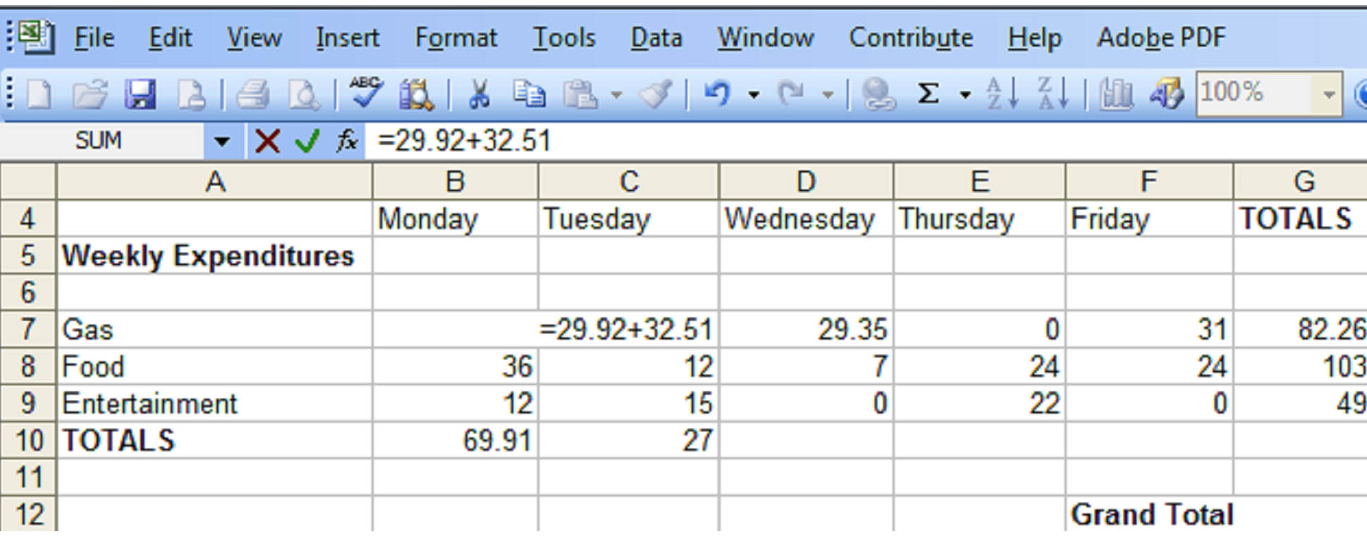
The equation appears in the formula bar as well as in the individual cell as you type it. Hit Enter and the equation disappears, leaving only the sum of the two numbers: 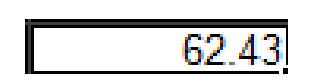 . If you want to see the formula again, click on the cell. The formula will be visible in the formula bar.

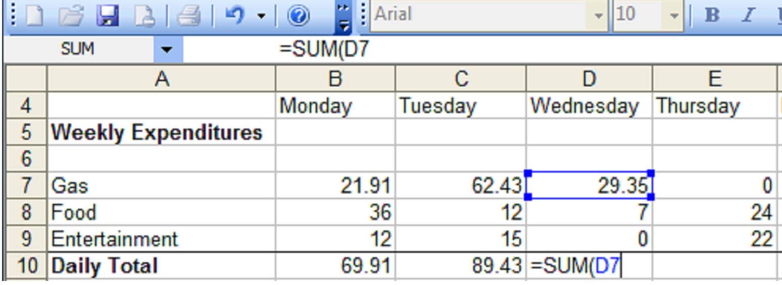
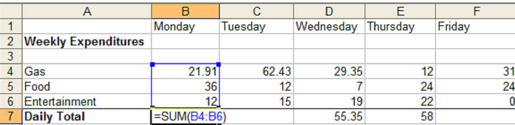
You can also perform a calculation based on the values within a series of cells. Let's add up the figures in column D. The individual cell coordinates are D7, D8, and D9. We want the total to appear in cell D10, in the row called Daily Total. Select that cell and verify your selection by checking the Name Box.
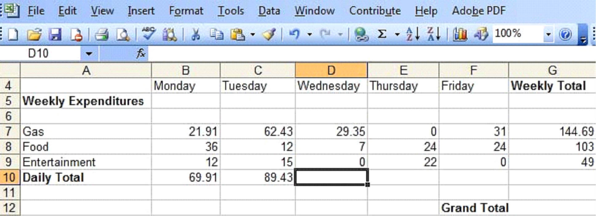
Now we'll type =SUM(D7:D9). The equals sign tells MS Excel that you are going to enter a formula. The SUM tells it to add the following numbers and the colon tells it the range (D7 to D9. )
You'll notice that as you type D7, the text changes color (in this case blue) and the cell D7 becomes outlined in that color as well. This gives you a visual representation of the selected range.
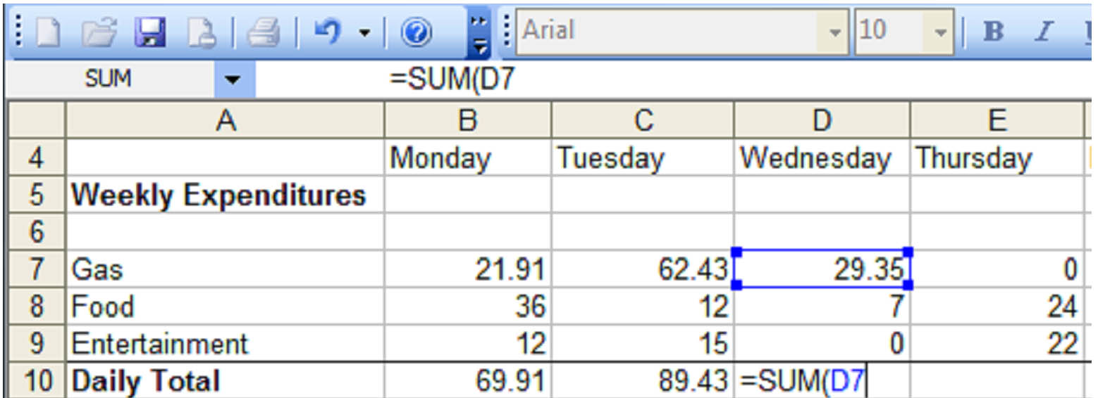
At this point, instead of typing D9, you could simply use the mouse to drag the lower edge of the blue box to D9. Excel will automatically enter the range symbol ( : ) and the cell name.
Hit Enter and the sum will appear in cell D10:
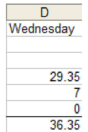
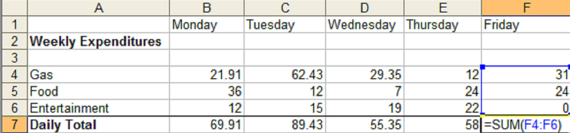
Because the sum depends upon the numbers in cells D7 thru D9, MS Excel will automatically recalculate the sum whenever the values of those cells change:
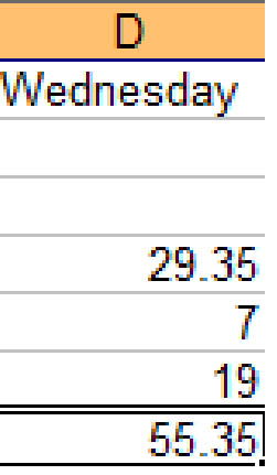
In the second example, you can see that we changed the value in cell D9 from "0" to "19." MS Excel finds the new sum automatically: "55.35".
References
Now let's take a closer look at references. A reference simply tells MS Excel where to find the information you want to use in a formula. As you've already learned, by default MS Excel uses the A1 reference style, or coordinate system, to identify cells. You can use these coordinates for references (as in the example above) or you can use labels and names.
Using labels and names makes it easier to understand the information you are entering into the formula. For instance, the formula "=SUM(WednesdayTotal)" is easier to understand than "=SUM(D7:D9)
Using Labels
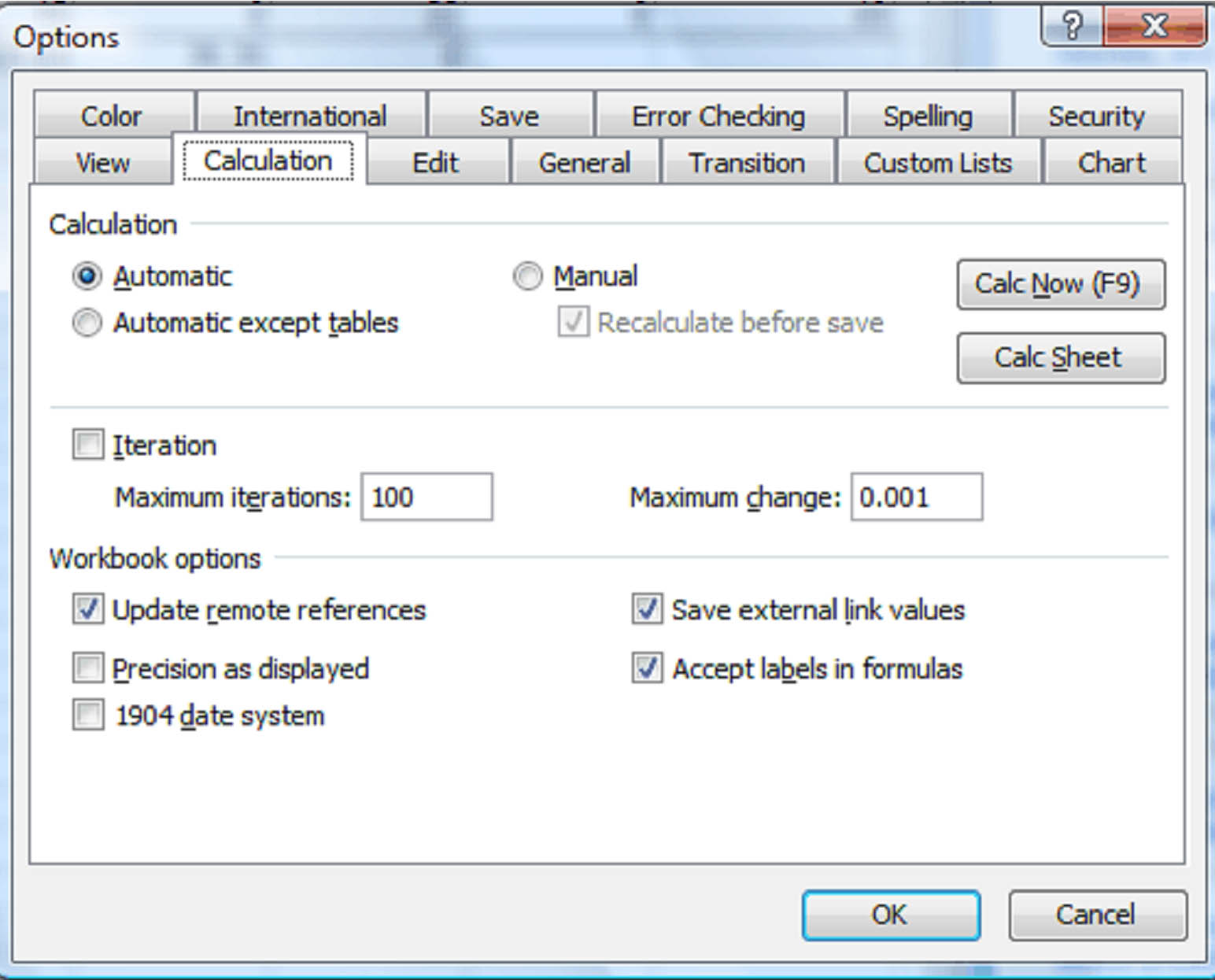
A label is used to identify a range of cells. For example, the word "Thursday" in cell E4 can be used to represent all the cells in column D. Likewise, the word "Gas" can be used to represent all of the cells in row 7. To use a label in a formula, you must first turn on the feature, which is turned off by default.
To turn it on click Tools > Options, then select the Calculations tab. Click the box beside "Accept labels in formulas" to select it.
A drawback to using labels, is that they can only be used to represent a range on the same worksheet. If you want to represent a range across multiple worksheets or even in another workbook, you must use a name.
Note: When a name for a formula or range is used in another workbook, it is called a "link."
Using Names
Unlike labels, names can represent more than just a range of cells. They can represent an unchanging number (called a constant) or even a formula. For instance, let's say sales tax is 8 percent. Since this number will not change between worksheets or workbooks, we can give it a name. In this case, we'll call it SalesTax.
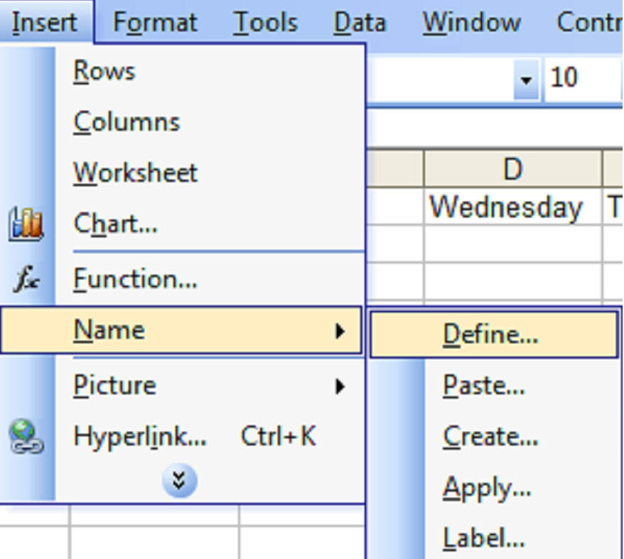
First, we'll want to define our name. We'll do this by clicking Insert > Name > Define:
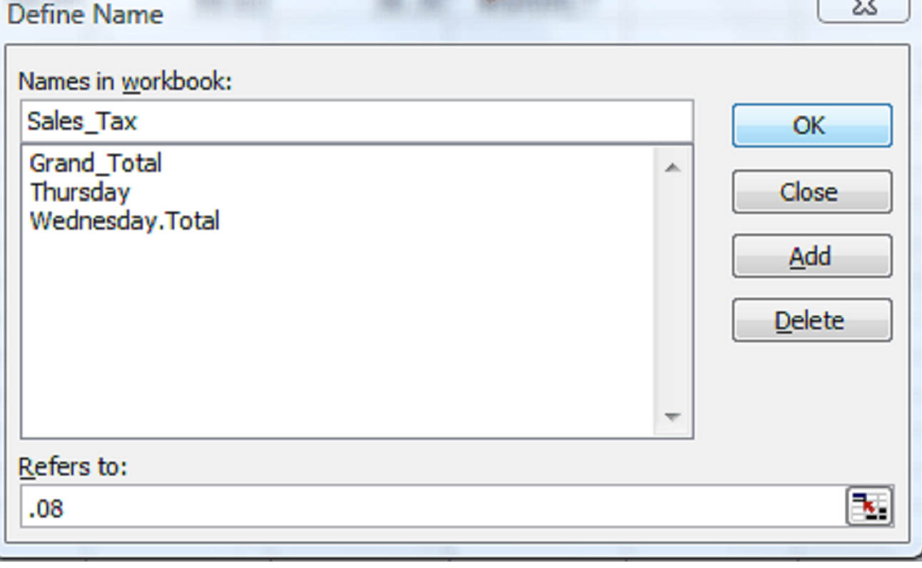
In the Define Name dialog box, we'll type Sales_Tax in the name window and .08 to represent 8 percent in the Refers to: box. Then click OK.
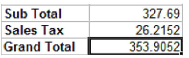
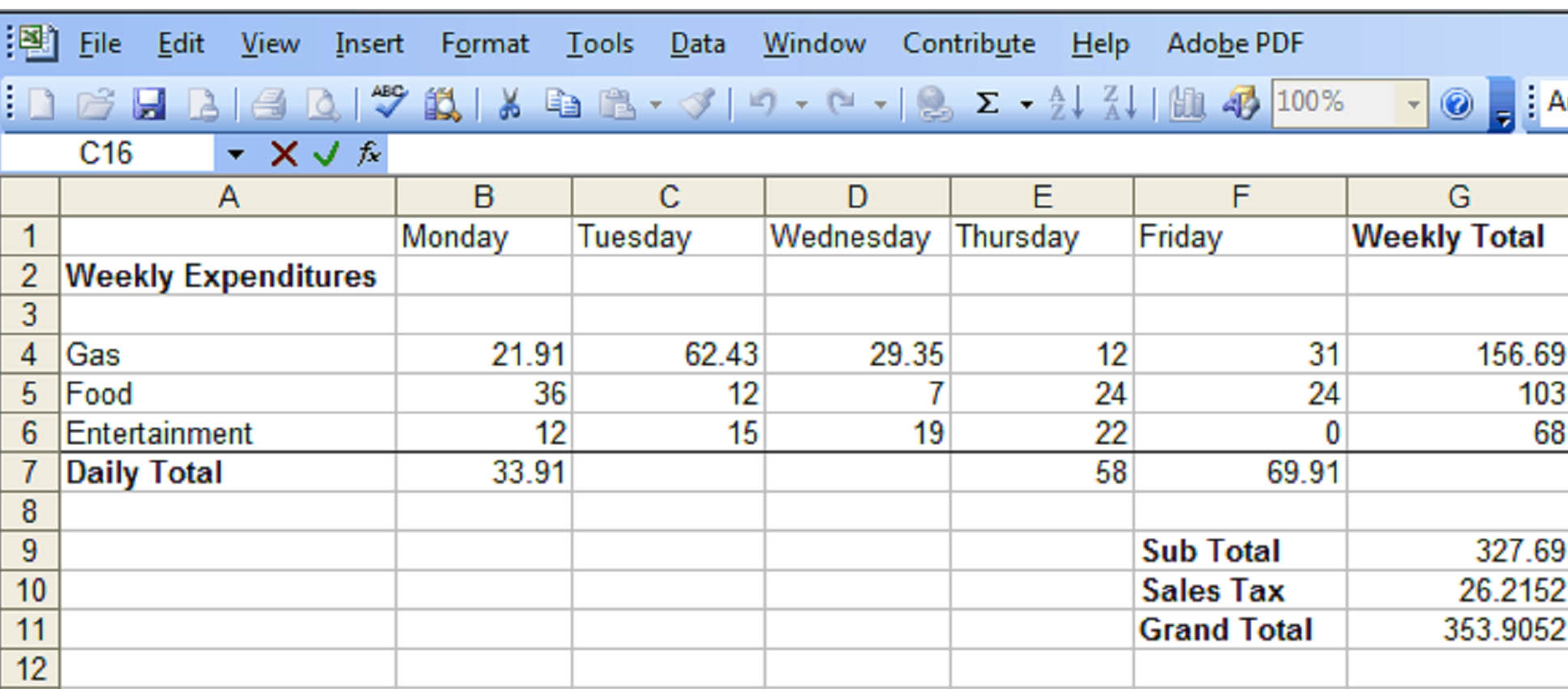
We now have a reference for sales tax. We can then use that reference in a formula. In the example below, we'll apply sales tax to the sub total (which we've already given a name: Sub_Total).
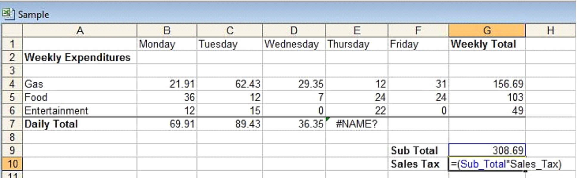
Since we've already attributed a name to cell G9, we will use it in our formula: "=(Sub_Total*Sales_Tax)". As you can see in the above example, the word "Sub_Total" and the cell it refers to (G9) are highlighted in blue while the word "Sales_Tax" is not. This is to give you a visual reminder of what the name refers to. Hit enter, and the product of 308.69 x .08 will appear in cell G10.
Let's say we wanted to add the sub total to the sales tax for a grand total and use the grand total as reference on worksheet 2. First we'd create a cell for the grand total and enter our formula:
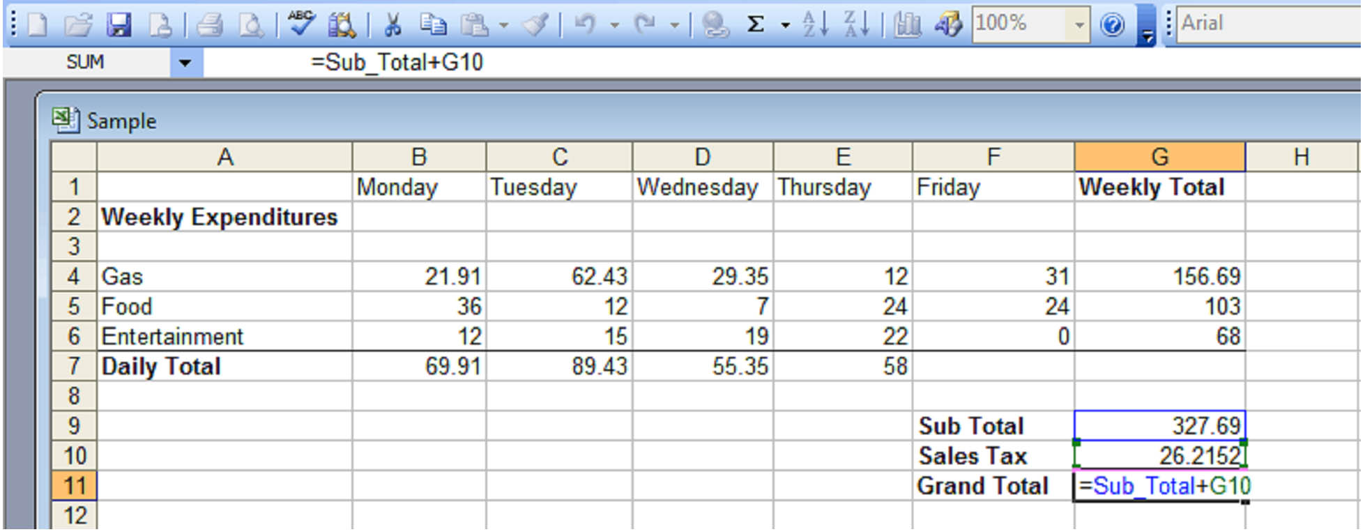
When we push Enter the sum of the Sub Total and Sales Tax will appear in cell G11:
There are two ways to use value on another worksheet. First, we can simply select the appropriate cell on the second worksheet and enter this into our formula:
"=Sheet1!$G$11".
As you've no doubt deduced, "Sheet1" in our formula tells Excel from which worksheet you want to select cell G11. Since each worksheet uses the A1 reference style, if you didn't use this, MS Excel would simply use the information in cell G11 in the current worksheet.
So if we wanted to add the grand total in worksheet1 to the grand total in worksheet2, the formula would look something like this:
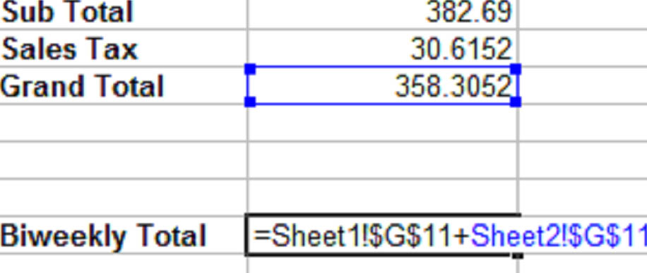
Because we're referring to a cell on the current worksheet, that cell and its reference are highlighted.
The dollar sign symbol ( $ ) represents an Absolute Reference, which we'll talk about in the next section.
But first, we'll use names to perform the same calculation. So let's go back and rename the value in cell G11 on worksheet1 "Grand_Total_Week1" and the value in cell G11 on worksheet2 "Grand_Total_Week2".
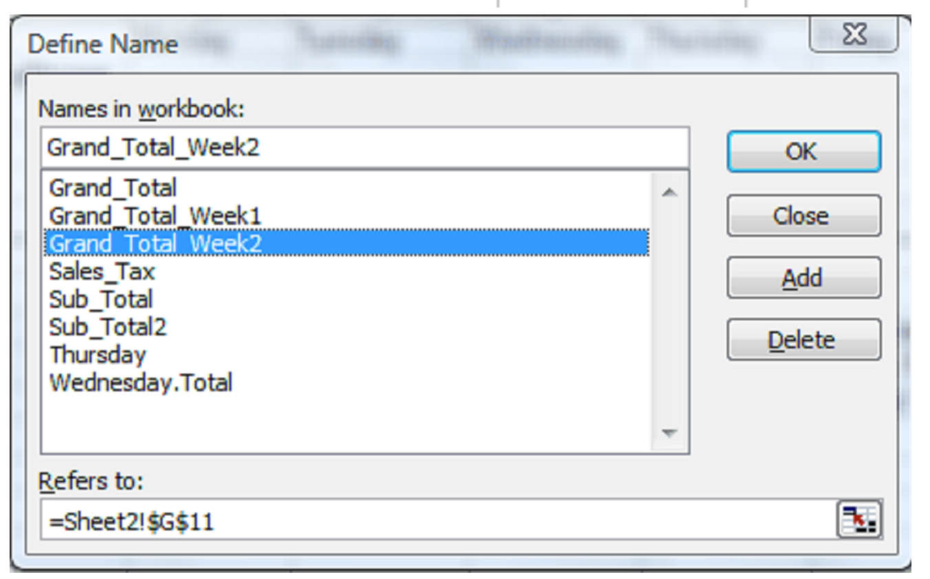
We can then just enter the names into our formula:
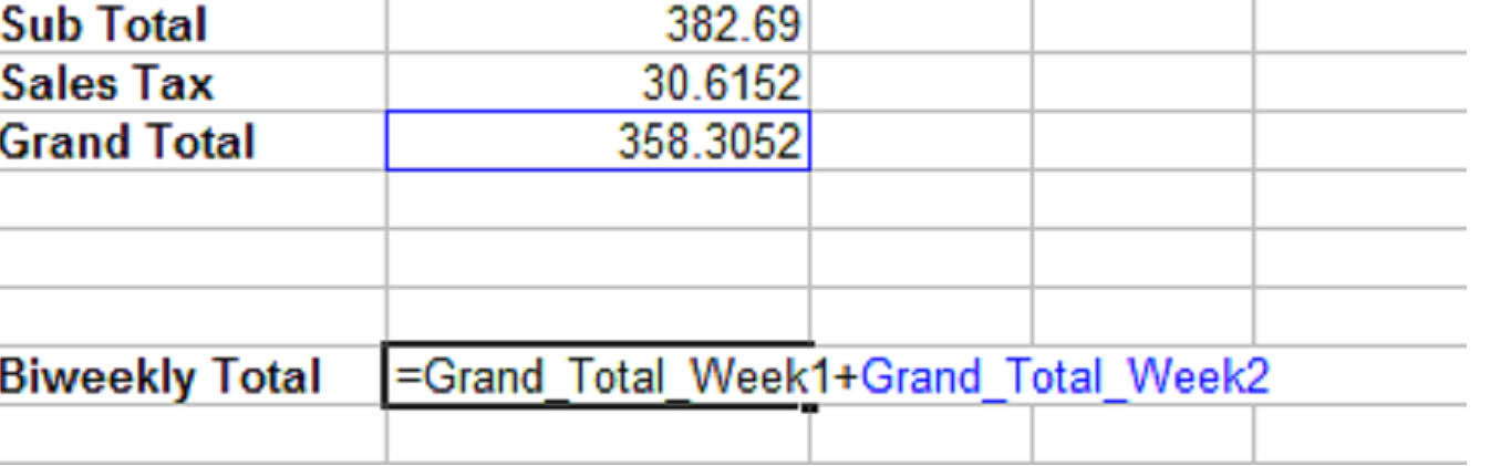
We could also give our formula a name:
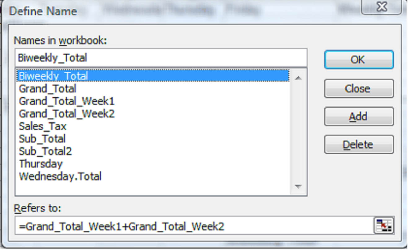
In this case, we've decided to call the formula "Biweekly_Total" and told MS Excel that the formula for "Biweekly_Total" is "Grand_Total_Week1+Grand_Total_Week2".
We can now select cell G15 on worksheet2 and type "=Biweekly_Total":
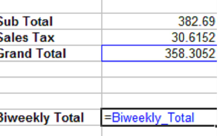
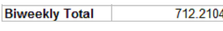
Press Enter and the MS Excel performs the calculations for you:
Absolute, Relative and Mixed Cell References
There are two kinds of cell references; Absolute and Relative.
A relative reference in a formula depends upon its position in a worksheet. For instance, the cell coordinates in the following example "B4:B6" are relative references.
If we copy the formula "=SUM(B4:B6)" from cell B7 in worksheet1 to cell F7 in worksheet1, the formula remains the same, but the cell references (B4:B6) change:
This is because MS Excel recognizes the relationship between the formula in cell B7 and its cell range (B4:B6). When we paste the formula into a new cell, it creates the same relationship in the new position.
An Absolute Reference does not depend upon its position in a worksheet. For instance, if the value in cell B7 were an absolute reference, when we pasted the formula in cell F7, the formula would read: =SUM($B$4:$B$6).
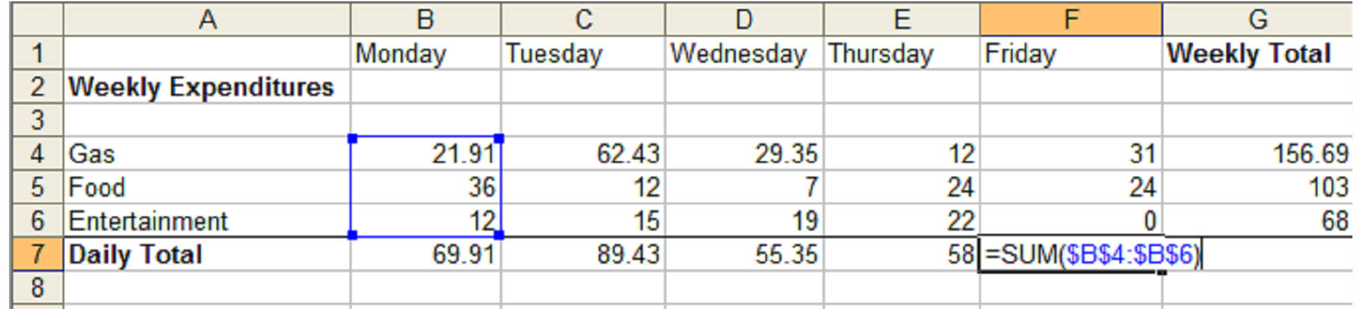
The symbol "$" in cell coordinates tells MS Excel that this is an absolute reference. Before we copied the formula from B7 to F7 in the example above, we changed it to an absolute reference by adding $'s: =SUM($B$4:$B$6). The blue box around cells B4 thru B6 and the blue cell coordinates in the formula, show us the relationship between the typed reference the cells. When we push enter, of course, we get 69.91 in cell F7.
A Mixed Reference contains both an absolute reference and a relative reference. Which means, it can either contain an absolute column and a relative row, or a relative column and an absolute row.
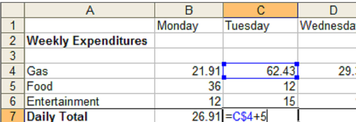
The reference $B4 is a mixed reference. Column B is absolute, while row 4 is relative. So when you change the position of the cell that contains the formula, the relative reference will change, but the absolute reference will not.
In the following example, we've created an mixed reference "=B$4+5":
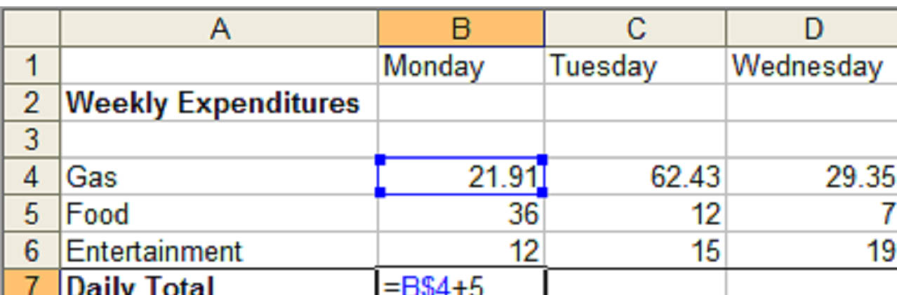
Our relative reference is for column B and our absolute reference is row 4. If we copy the formula to C7, the column changes but the row does not:
Functions
By now you've probably noticed the Insert Function button next to the formula bar:
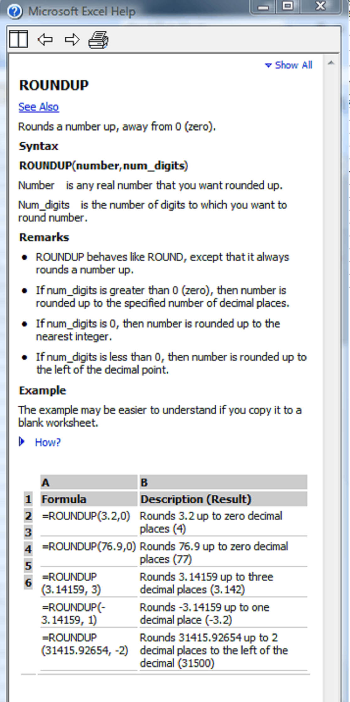
Functions are predefined formulas that perform calculations based upon specific values, called arguments. They can perform simple tasks, such as rounding off a number, or complex tasks like returning the inverse hyperbolic cosine of a number. (If your palms just got sweaty, don't worry, inverse hyperbolic cosines will not be mentioned again in this course.)
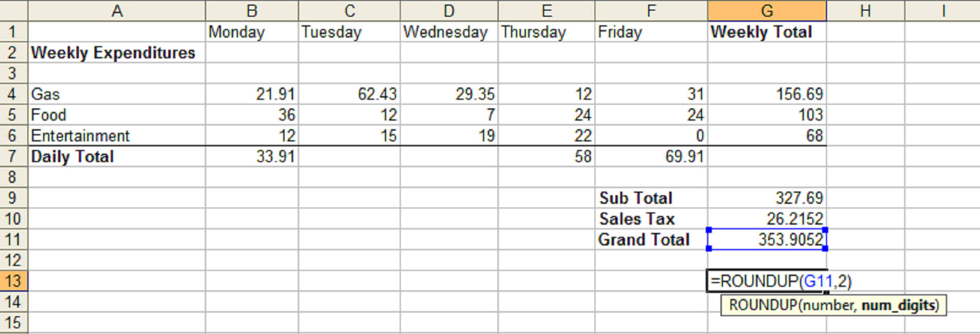
Let's look at a simple task. The following function will round the figure in cell G11 up two digits:
=ROUNDUP(G11,2)
A function, like a formula, always begins with an equals sign: =. This is followed by the function name. In this case, it's ROUNDUP. Next is the argument (G11,2). The argument is always enclosed in parenthesis. An argument gives the formula specific parameters. For instance, in our example, we're telling Excel we want to round up the value in cell G11 by two digits.
An argument can be a number, text, a logical value, an array or a cell reference.
When you enter a function, you'll see the tool tip box appear under it. If you need an explanation for any part of a function, just click on any word in the tool tip.
Note: Tool tips are only available for built-in functions.
In the above example, we clicked the word "ROUNDUP" in the tool tip.
Using Functions
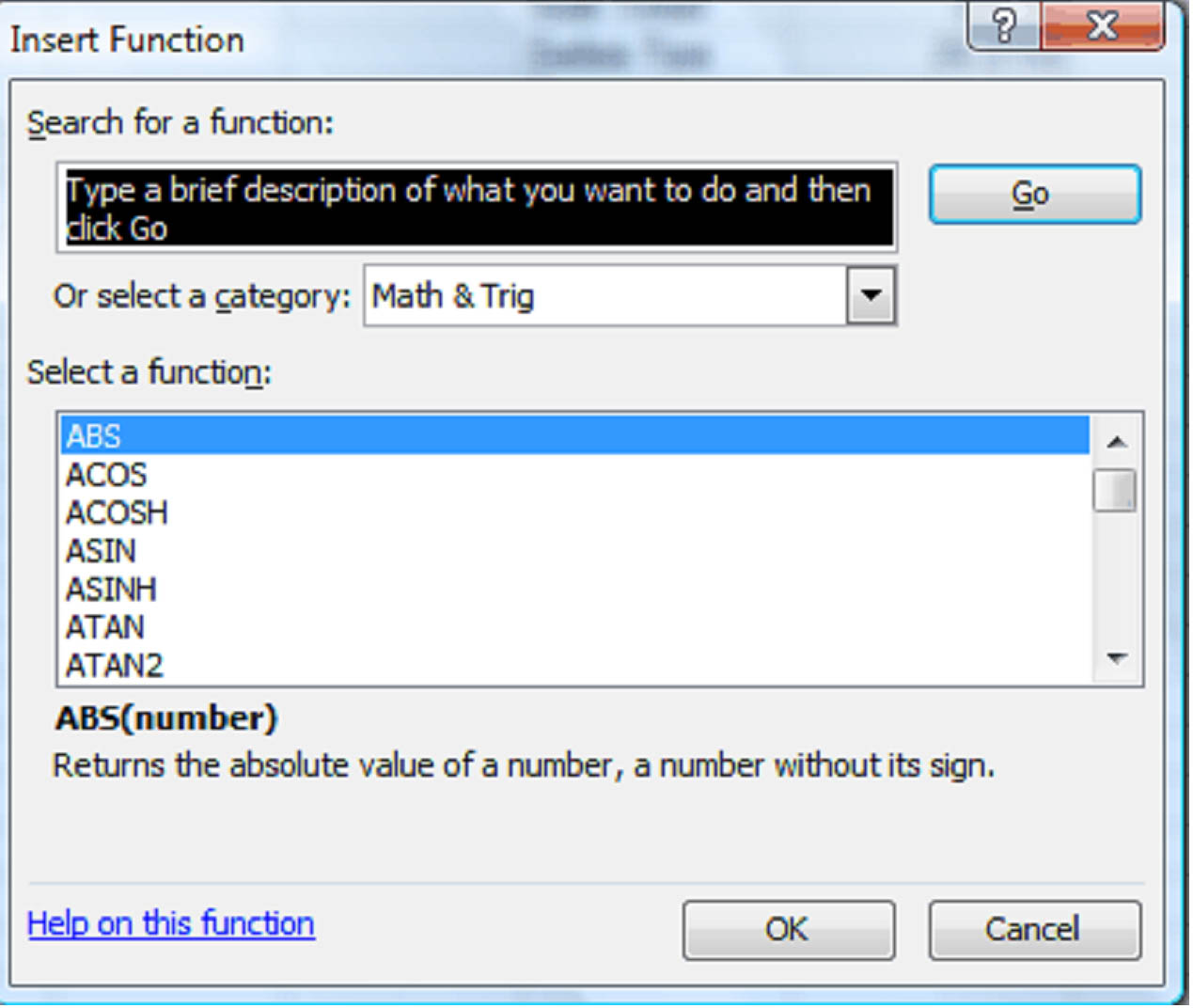
There are two ways to enter a function. If you know the function name and the syntax, you can select a cell and start typing. If you're not sure of its name, select a cell then click the function button .
This is what you will see:
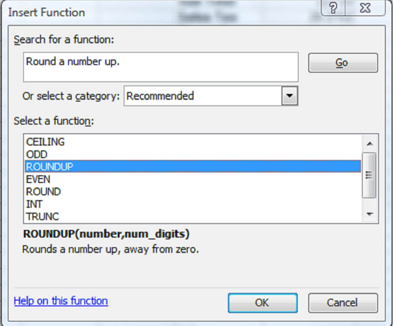
If you have a pretty good idea of what you want to do, select the "Search for a function" box and start typing. In our case, we want to round a number up. So we'll type "Round a number up" and click Go.
Excel searches the description for each function and comes up with a list of close matches. You can see what each function does, by selecting it. In the above example, we've selected ROUNDUP. The function and its syntax appears below the "Select function" box, as well as its description. Click OK.
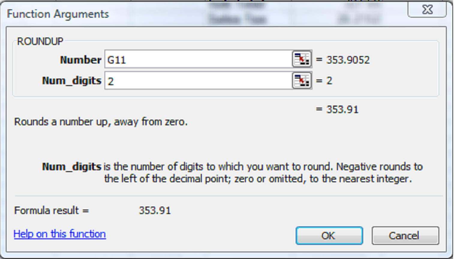
The Function Arguments dialog will open. Type the number or reference you want to round up in the number box. Since we want to round up the value of cell G11, we'll enter that into the Number box. If you're not sure what value to enter, just click the box. An explanation will appear below. In this example, the Num_digits box is selected. We can see its explanation in the lower middle of the box:
We want to round the number up two digits, so we enter that figure into the Num_digits box and click OK. The formula result (353.91) in this case, appears in the selected cell in our worksheet.
If you know what kind of calculation you want Excel to perform, but you're not quite sure how to articulate it, you can browse through the functions in the Insert Function dialog box. Just scroll through the list and select the one that seems the most appropriate. You can narrow the search results by choosing a category in the "Or select a category" box.
So now you've learned all about formulas and functions.